Feature-Interactions Based Information Retrieval Models

Introduction

Large-scale information retrieval applications, such as recommender systems, search ranking, and text analysis often leverage feature interactions for effective modeling. These models are commonly deployed at the ranking stage of the cascade-style systems. In this article, I summarize the need for modeling feature interactions and introduce some of the most popular ML architectures designed around this theme. This article also highlights the high data sparsity issue, that makes it hard for ML algorithms to model second or higher-order feature interactions.

Why Should We Model Feature Interactions?

As an example, consider an artificial Click-through rate (CTR) dataset shown in the table below, where + and - represent the number of clicked and unclicked impressions respectively.

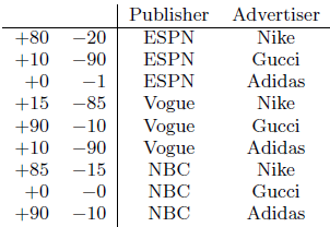
We can see that an ad from Gucci has a high CTR on Vogue. It is difficult for linear models to learn this information because they learn the two weights Gucci and Vogue separately. To address this problem, a machine learning model will have to learn the effect of their feature interaction. Algorithms such as Poly2 (degree-2 polynomial) do this by learning a dedicated weight for each feature conjunction ($O(n^{2})$ time complexity).

Order of Interaction

An order-2 interaction can be between two features, such as app category and timestamp. For example, people often download Uber apps for food delivery at meal-time. Similarly, an order-3 interaction can be between app category, user gender, and age. For example, a report showed that male teenagers like shooting and RPG games. Some research works argue that considering low- and high-order feature interactions simultaneously brings additional improvement over the cases of considering either alone¹. For a highly sparse dataset, these feature interactions are often hidden and difficult to identify a priori.

Data Sparsity

A variety of information retrieval and data mining tasks, such as recommender systems, targeted advertising, etc. model discrete and categorical variables extensively. As an example, these variables could be user demographics such as gender and occupation, or item categories. Additionally, these systems also utilize identifiers like user IDs, product IDs, and advertisement IDs. A common technique for using these categorical variables in machine learning algorithms is to convert them to a set of binary vectors via one-hot encoding. This means that for a system with a large (millions, or even billions) userbase and item catalog, the resultant feature input is highly sparse as the actual engagement data is comparatively smaller.

This highly sparse data makes it difficult to learn effective feature interactions because often there isn’t any observed data for a lot of combinations of feature values. For example, there is no training data for the pair (NBC, Gucci) in the table above.

Memorization vs Generalization Paradigm

One common challenge in building such applications is to achieve both memorization and generalization.

• Memorization is about learning the frequent co-occurrence of features and exploiting the correlations observed from the historical data. As an example, the Google Play store recommender system might use two features ‘installed_app’ and ‘impression_app’ to calculate the probability of a user installing the ‘impression_app’. Memorization-based algorithms use cross-product transformation and look at specific features, such as “AND(previously_installed_app=netflix, current_impression_app=spotify)”, whose value is 1, and correlate it with the target label.

  While such recommendations are topical and directly relevant based on the user’s previous actions, they can not generalize when cross-feature interaction never happened in the training data, like the (NBC, Gucci) pair in the table above. Creating cross-product transformations may also require a lot of manual feature engineering effort.

• Generalization is based on the transitivity of correlation and exploring new feature combinations that have never or rarely occurred in the past. To achieve this generalization we use embeddings-based methods, such as factorization machines or deep neural networks by learning a low-dimensional dense embedding vector.

  While such recommenders tend to improve the diversity of the recommended items, they also suffer from the problem of over-generalizing for cases such as users with specific preferences, or niche items with a narrow appeal. Also, dense embedding methods always lead to nonzero predictions and thus make less relevant recommendations at times. Comparatively, it is easier for generalized linear models with cross-product feature transformations to memorize these “exception rules” for unique users and items with much fewer parameters.

Model Architectures

In this article, I will introduce, implement and compare seven popular model architectures that try to balance both memorization and generalization to some degree. Each of the model implementations is done in its standalone Jupyter Notebook file and is linked in the corresponding section below. Every notebook contains code for data preprocessing, model definition, training, and evaluation as applicable to the respective model.

1. Factorization Machine (FM)

Factorization Machines (FMs) were originally purposed in 2010 as a supervised machine-learning method for collaborative recommendations. FMs allow parameter estimation under very sparse data where its predecessors, like SVMs failed, and unlike Matrix Factorization it isn’t limited to modeling the relation of two entities only. FMs learn second-order feature interactions on top of a linear model by modeling all interactions between each pair of features. They can also be optimized to work in linear time complexity. While in principle, FM can model high-order feature interaction, in practice usually only order-2 features are considered due to high complexity.

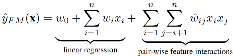
where $w_{0}$ is the global bias, $w_{i}$ denotes the weight of the i-th feature, and $ŵ_{ij}$ denotes the weight of the cross feature $x_{i}x_{j}$, which is factorized as: $ŵ_{ij} = v_{i}^{T} v_{j}$, where $v_{i} \in R^{k}$ denotes the embedding vector for feature i, and k denotes the size of the embedding vector.

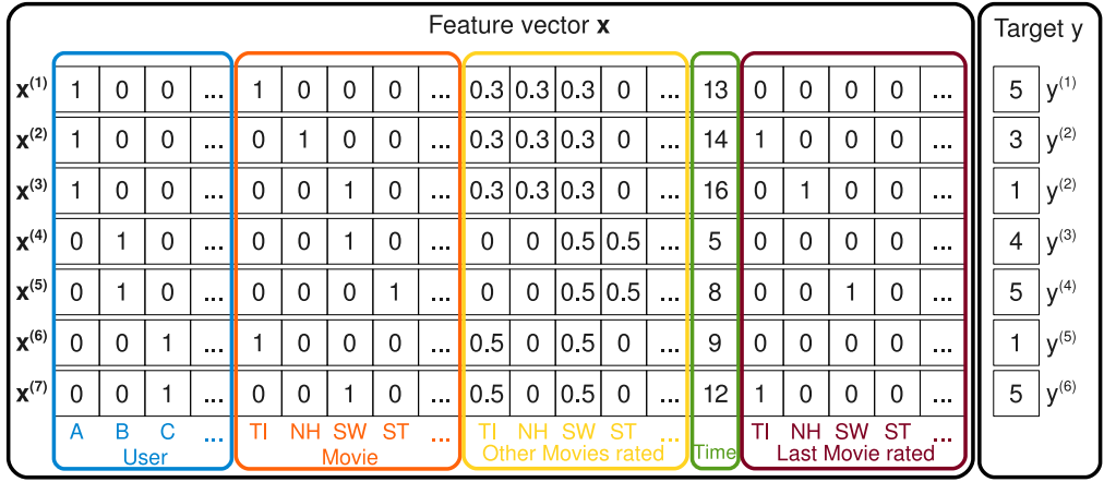
The example above shows a sparse input feature vector x with corresponding target y. We have binary indicator variables for the user, movie, and the last movie rated, along with a normalized rating for other movies and timestamps. Let’s say we want to estimate the interaction between the user Alice (A) and the movie Star Trek (ST). You will notice that we do not have any example in x with an interaction between A and ST. FM can still estimate this by using the factorized interaction parameters $\langle v_{A}, v_{ST} \rangle$ even in this case.

Implementation

Suppose we have M training examples, n features and we want to factorize feature interaction with vectors of size k i.e. dimensionality of $v_{i}$. Let us denote our trainset as $X \in R^{M×n}$, and matrix of $v_{i}$ (the ith row is $v_{i}$) as $V \in R^{n×k}$. Also, let’s denote the feature vector for the jth object as $x_{j}$. So:

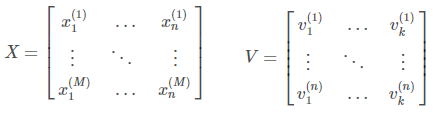
The number in brackets indicates the index of the sample for x and the index of the feature for v. Also, the FM equation can be expressed as:

$S_{1}$ is a dot product of feature vector $x_{j}$ and ith column of V. If we multiply X and V, we get:

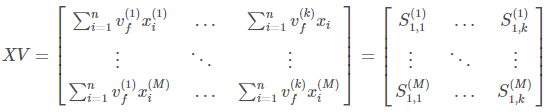
So if square XV element-wise and then find the sum of each row, we obtain a vector of $S_{1}^{2}$ terms for each training sample. Also, if we first square X and V element-wise, then multiply them, and finally sum by rows, we’ll get $S_{2}$ term for each training object. So, conceptually, we can express the final term like this:

PyTorch Code

Refer to this Gist for the complete code for this experiment: https://gist.github.com/reachsumit/2a639276fc781870c4dcd480a3417bf9

You can read more about FMs in the original paper and the official codebase.

2. Field-Aware Factorization Machine (FFM)

Let’s revisit the artificial dataset example from earlier and add another column Gender to it. One observation of such a dataset might look like this:

FMs will model the effect of feature conjunction as: $w_{ESPN} \cdot w_{Nike} + w_{ESPN} \cdot w_{Male} + w_{Nike} \cdot w_{Male}$. Field-aware factorization machines (FFMs) extend FMs by introducing the concept of fields and features. With the same example, Publisher, Advertiser, and Gender will be called fields, while values like ESPN, Nike, and Male will be called their features. Note that in FMs every feature has only one latent vector to learn the latent effect with any other features. For example, for ESPN $w_{ESPN}$ is used to learn the latent effect with Nike ($w_{ESPN} \cdot w_{Nike}$) and Male ($w_{ESPN} \cdot w_{Male}$). However, because Nike and Male belong to different fields, the latent effects of (EPSN, Nike) and (EPSN, Male) may be different.

In FFMs, each feature has several latent vectors. Depending on the field of other features, one of them is used to do the inner product. So, for the same example, the feature interaction effect is modeled by FFM as: $w_{ESPN,A} \cdot w_{Nike,P} + w_{ESPN,G} \cdot w_{Male,P} + w_{Nike,G} \cdot w_{Male,A}$. To learn the latent effect of (ESPN, NIKE), for example, $w_{ESPN,A}$ is used because Nike belongs to the field Advertiser, and $w_{Nike,P}$ is used because ESPN belongs to the field Publisher.

If f is the number of fields, then the number of variables of FFMs is nfk, and the time complexity is $O(\bar{n}^{2}k)$. Note that because each latent vector in FFMs only needs to learn the effect with a specific field, usually: $k_{FFM} \ll k_{FM}$. FFM authors empirically show that for large, sparse datasets with many categorical features, FFMs perform better than FMs. Whereas for small and dense datasets or numerical datasets, FMs perform better than FFMs.

Implementation

PyTorch Code

Refer to this Gist for the complete code for this experiment: https://gist.github.com/reachsumit/c6a8037f4596a8181376313fdba33ffd

You can read more about FFMs in the original paper and the official codebase.

3. Attentional Factorization Machine (AFM)

However, despite its effectiveness, FMs model all feature interactions with the same weight, but not all feature interactions are equally useful and predictive. For example, the interactions with useless features may even introduce noise leading to degraded model performance. Attentional Factorization Machines (AFMs) fix this by learning the importance of each feature interaction from data via a neural attention network.

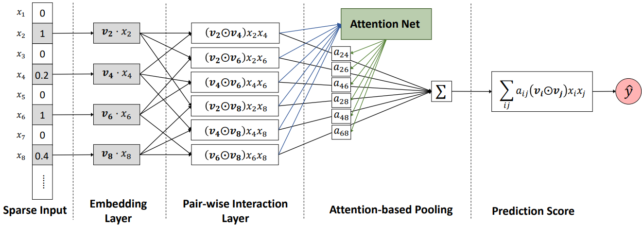
AFM starts with sparse input and embedding layer and inspired by FM’s inner product, it expands m vectors to $\frac{m(m-1)}{2}$ interacted vectors, where each interacted vector is the element-wise product of two distinct vectors to encode their interaction. The output of the pair-wise interaction layer is fed into an attention-based pooling layer, the idea here is to allow different parts to contribute differently when compressing them to a single representation. An attention mechanism is applied to feature interactions by performing a weighted sum on the interacted vectors. This weight or attention score can be thought of as the importance of weight $\hat{w}_{ij}$ in predicting the target. One shortcoming of AFM architecture is that it models only second-order feature interactions.

Implementation

PyTorch Code

Refer to this Gist for the complete code for this experiment: https://gist.github.com/reachsumit/85fe046691c66221bec00bc7e59e145b

You can read more about AFMs in the original paper and the official codebase.

4. Wide & Deep Learning

The Wide & Deep learning framework was proposed by Google to achieve both memorization and generalization in one model, by jointly training a linear model component and a neural network component. The wide component is a generalized linear model to which raw input features and transformed features (such as cross-product transformations) are supplied. The deep component is a feed-forward neural network, which consumes sparse categorical features in embedding vector form. The wide and deep parts are combined using a weighted sum of their output log odds as the prediction which is then fed to a common loss function for joint training.

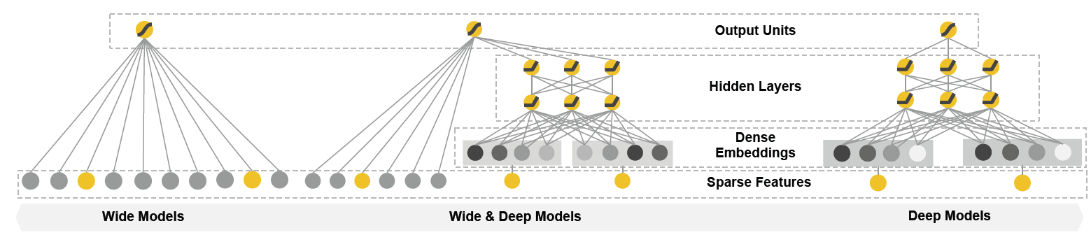
The authors claim that wide linear models can effectively memorize sparse feature interactions using cross-product feature transformations, while deep neural networks can generalize to previously unseen feature interactions through low-dimensional embeddings. Note that the wide and deep parts work with two different inputs and the input to the wide part still relies on expertise feature engineering. The model also suffers from the same problem as the linear models like Polynomial Regression that feature interactions can not be learned for unobserved cross features.

Implementation

PyTorch Code

Refer to this Gist for the complete code for this experiment: https://gist.github.com/reachsumit/a6ab97ed6bc053aaf3d73320b4b31b97

You can read more about Wide&Deep in the original paper and the official codebase.

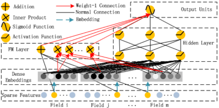
5. DeepFM

DeepFM model architecture combines the power of FMs and deep learning to overcome the issues with Wide&Deep networks. DeepFM uses a single shared input to its wide and deep parts, with no need for any special feature engineering besides raw features. It models low-order feature interactions like FM and models high-order feature interactions like DNN.

Implementation

PyTorch Code

Refer to this Gist for the complete code for this experiment: https://gist.github.com/reachsumit/79237a4de62b4033e2576c55df3dc056

You can read more about DeepFM in the original paper.

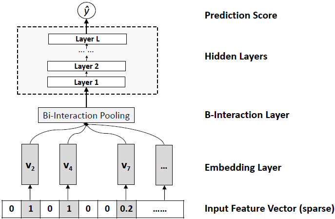
6. Neural Factorization Machine (NFM)

Neural Factorization Machine (NFM) model architecture was also proposed by the authors of the AFM paper with the same goal of overcoming the insufficient linear modeling of feature interactions in FM. After the sparse input and embedding layer, this time the authors propose a Bi-Interaction layer that models the second-order feature interactions. This layer is a pooling layer that converts a set of the embedding vectors set input to one vector by performing an element-wise product of vectors: $\sum_{i=1}^{n} \sum_{j=i+1}^{n} x_{i}v_{i} \odot x_{j}v_{j}$, and passes it on to another set of fully connected layers.

Implementation

PyTorch Code

Refer to this Gist for the complete code for this experiment: https://gist.github.com/reachsumit/f29d7001b7687785f33636c9bca302c3

You can read more about NFM in the original paper and the official codebase.

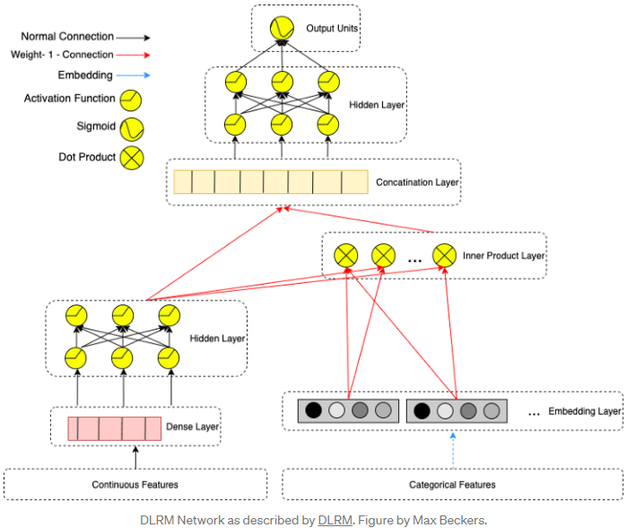
7. Deep Learning Recommendation Model (DLRM)

The Deep Learning Recommendation Model (DLRM) was proposed by Facebook in 2019. The DLRM architecture can be thought of as a simplified version of DeepFM architecture. DLRM tries to stay away from high-order interactions by not passing the embedded categorical features through an MLP layer. First, it makes the continuous features go through a “bottom” MLP layer such that they have the same length as the embedding vectors. Then, it computes the dot product between all combinations of embedding vectors and the bottom MLP output from the previous step. The dot product output is then concatenated with the bottom MLP output and is passed to a “top” MLP layer to compute the final output.

This architecture design is tailored to mimic the way Factorization Machines compute the second-order interactions between the embeddings, and the paper also says:

We argue that higher-order interactions beyond second-order found in other networks may not necessarily be worth the additional computational/memory cost.

Implementation

The paper also notes that DLRM contains far more parameters than common models like CNNs, RNNs, GANs, and transformers, making the training time for this model go up to several weeks. They also propose a framework to parallelize DLRM operations. Due to high compute requirements, I couldn’t train the DLRM model myself. DLRM results in this experimentation are with a simplified implementation using a concatenation of bottom MLP output and embedding output, instead of their dot product.

PyTorch Code

Refer to this Gist for the complete code for this experiment: https://gist.github.com/reachsumit/a02a83fbb3ae5e293fde4b90e3a319d7

You can read more about DLRM in the original paper and the official codebase.

Toy Experiment

Dataset Preprocessing

For this article, I will be using the MovieLens 100K dataset² from Kaggle. It contains 100K ratings from 943 users on 1682 movies, along with demographic information for the user. Each user has rated at least 20 movies. The following transformations were applied to prepare the dataset for experimentation.

• The dataset was sorted by user_id and timestamp to create time ordering for each user.
• A target column was created which is time-wise the next movie that the user will watch.
• New columns such as average movie rating per user, average movie rating per genre per user, number of movies watched per user in each genre normalized by total movies watched by that user, etc. were created.
• The gender column was label encoded, and the occupation column was dummy encoded.
• Continuous features were scaled as appropriate.
• A sparse binary tensor was created indicating movies that the user has watched previously.
• The dataset was split into train-test with an 80-20 ratio.

The following diagram shows the various features generated through preprocessing. Some or all of these features are used during experimentation depending upon the specific model architecture.

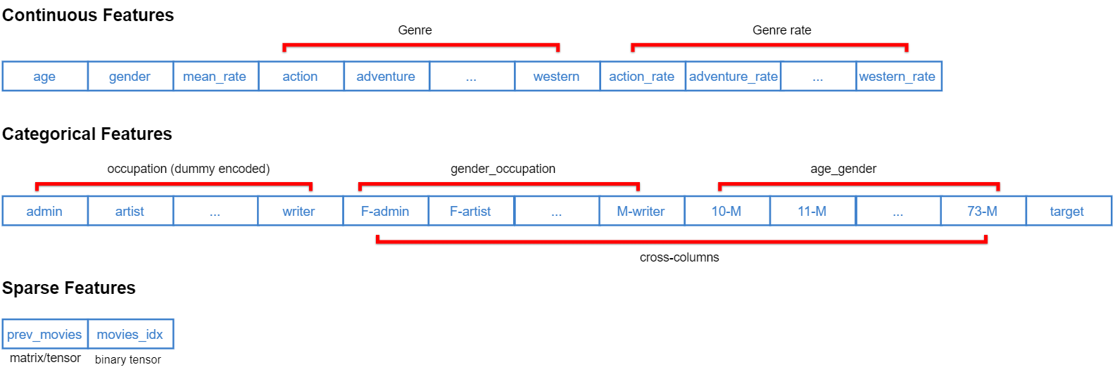
Refer to the respective notebook for data preprocessing steps specific to each model.

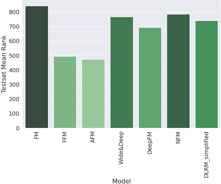
Comparison Results

The mean rank of the test set examples was computed using each model, and the following chart shows their comparison based on the best rank achieved on the test set. In short, for this experiment: AFM > FFM » DeepFM > DLRM_simplified > Wide & Deep > NFM > FM.

Summary

In this article, we defined the need for modeling feature interactions and then looked at some of the most popular machine-learning algorithms designed to estimate feature interactions under sparse settings. We implemented all of the algorithms in Python and compared their results on a toy dataset.

References