Collaborative Filtering based Recommender Systems for Implicit Feedback Data

Different Flavors of Recommenders

At a high-level, Recommender systems work based on two different strategies (or a hybrid of the two) for recommending content.

• Collaborative Filtering: Algorithms that use usage data, such as explicit or implicit feedback from the user.
• Content-based Filtering: Algorithms that use content metadata and user profile. For example, a movie can be profiled based on its genre, IMDb ratings, box-office sales, etc., and a user can be profile based on their demographic information or their answers to an onboarding survey.

So, while collaborative filtering needs much feedback from the users to work properly, content-based filtering needs good descriptions of the items.

Challenges With Using Explicit Data

Broadly speaking, the usage data can be either an explicit or implicit signal from the user. Explicit feedback is likely the most accurate input for the recommender system because it is pure information provided by the user about their preference for certain content. This feedback is usually collected using controls such as upvote/downvote buttons or star ratings.

Despite their flaws, explicit feedback is used by a vast majority of recommender systems probably thanks to the convenience of using such an input.

However, explicit feedback is not always available and often lacks nuances. Not everyone who purchases a product on Amazon or watches a movie on Netflix likes to leave feedback, people might rate a product lower because of their bad experience with an Amazon delivery agent, and someone might rate a movie higher not because of the content of the movie but simply because they liked the movie’s cover art.

Explicit feedback collection is not even possible for products like movies or shows broadcasted on television. Similarly, a platform may not have a feedback system with 0 or negative ratings, so if you don’t like a product, the lowest rating you can give to it might still be a 1-star. This dilutes how strongly you may dislike the product, and for the recommender system, it means that the dataset lacks substantial evidence on which products consumers dislike.

Despite their flaws, explicit feedback is used by a large number of recommender systems probably thanks to the convenience of using such an input. The missing information is simply considered as empty cells in a sparse matrix input and is omitted from the analysis. Using explicit signals requires additional boosting algorithms to get user feedback on new content because collaborative filtering will not be able to recommend the new content until someone rates it (also known as the cold start problem).

Building a Recommender System Using Explicit Feedback

Before we talk about using implicit signals, let’s implement a collaborative filtering based recommender system using explicit signals. We will implement a matrix factorization based algorithm using NumPy’s SVD ¹ on MovieLens 100K dataset ². This dataset contains 100,000 ratings given by 943 users for 1682 movies, with each user having rated at least 20 movies.

Quick Notes on How Matrix Factorization Works

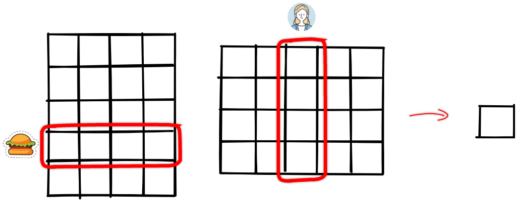
We start with a U x M rating matrix (943x1682 for our dataset) where each value $r_{ui}$ represents the rating given by user u for a movie i. We then divide this matrix into two much smaller matrices such that we approximately get the same U x M matrix back if we multiply the two new matrices together. Basically, we compress a high-dimensional sparse input matrix to a low-dimensional dense matrix space because this generalization leads to a better understanding of the data. Refer to Yehuda Koren’s paper to read more about how the matrix factorization technique is used for recommender systems ³. To learn how SVD works, refer to Jeremy Kun’s article on Math ∩ Programming ⁴.

By splitting this matrix into lower dimensions (factors), we represent each user as well as each movie by a 50-dimensional dense vector.

To recommend movies similar to a given movie, we can compute the dot product (cosine similarity) between that movie and other movies and take the closest candidates as the output. Alternatively, we can compute the dot product of a user vector u and an item vector i to get the predicted score and sort all unrated items’ predicted score for a given user to get the list of recommended items for a user.

Python Implementation

 1
 2
 3
 4
 5
 6
 7
 8
 9
10
11
12
13
14
15
16
17
18
19
20
21
22
23
24
25
26
27
28
29
30
31
32
33
34
35
36
37
38
39
40
41
42
43
44
45
46
47
48
49
50
51
52
53
54
55
56
57
58
59
60
61
62
63
64
65
66
67
68
69
70
71
72
73
74
75
76
77
78
79
80
81
82

import numpy as np
import pandas as pd

from numpy import bincount, log, log1p
from scipy.sparse import coo_matrix, linalg

class ExplicitCF:
    def __init__(self):
        self.df = pd.read_csv("ml-100k/u.data", sep='\t', header=None, names=['user', 'item', 'rating'], usecols=range(3))
        self.df['user'] = self.df['user'].astype("category")
        self.df['item'] = self.df['item'].astype("category")
        self.df.dropna(inplace=True)
        
        self.rating_matrix = coo_matrix((self.df['rating'].astype(float),
                                  (self.df['item'].cat.codes,
                                  self.df['user'].cat.codes)))
    
    def _bm25_weight(self, X, K1=100, B=0.8):
        """Weighs each row of a sparse matrix X  by BM25 weighting"""
        # calculate idf per term (user)
        X = coo_matrix(X)
        N = float(X.shape[0])
        idf = log(N) - log1p(bincount(X.col))
        # calculate length_norm per document (artist)
        row_sums = np.ravel(X.sum(axis=1))
        average_length = row_sums.mean()
        length_norm = (1.0 - B) + B * row_sums / average_length
        # weight matrix rows by bm25
        X.data = X.data * (K1 + 1.0) / (K1 * length_norm[X.row] + X.data) * idf[X.col]
        return X
    
    def factorize(self):
        item_factor, _, user_factor = linalg.svds(self._bm25_weight(self.rating_matrix), 50)
        return item_factor, user_factor
    
    def init_predict(self, x_factors):
        # fully normalize factors, so can compare with only the dot product
        norms = np.linalg.norm(x_factors, axis=-1)
        self.factors = x_factors / norms[:, np.newaxis]
    
    def get_related(self, x_id, N=5):
        scores = self.factors.dot(self.factors[x_id])
        best = np.argpartition(scores, -N)[-N:]
        print("Recommendations:")
        for _id, score in sorted(zip(best, scores[best]), key=lambda x: -x[1]):
            print(f"item id: {_id}, score: {score}")

cf_object = ExplicitCF()
print(cf_object.df.head())
#  user item  rating
#0  196  242       3
#1  186  302       3
#2   22  377       1
#3  244   51       2
#4  166  346       1
print(cf_object.df.user.nunique()) # 943
print(cf_object.df.item.nunique()) # 1682
print(cf_object.df.rating.describe())
#count    100000.000000
#mean          3.529860
#std           1.125674
#min           1.000000
#25%           3.000000
#50%           4.000000
#75%           4.000000
#max           5.000000
#Name: rating, dtype: float64
print(cf_object.rating_matrix.shape) # (1682, 943)

item_factor, user_factor = cf_object.factorize()
print(item_factor.shape) # (1682, 50)
print(user_factor.shape) # (50, 943)

cf_object.init_predict(item_factor)
print(cf_object.factors.shape) # (1682, 50)
cf_object.get_related(314)
#Recommendations:
#item id: 314, score: 1.0
#item id: 315, score: 0.8940031189407059
#item id: 346, score: 0.8509562164687848
#item id: 271, score: 0.8441764974934266
#item id: 312, score: 0.7475076699852435

Code is also available on this GitHub Gist.

Challenges With Using Implicit Data

Implicit user feedback includes purchase history, browsing history, search patterns, impressions, clicks, or even mouse movements. While with explicit feedback, the user specifies the degree of positive or negative preference for an item, we do not have the same symmetry with implicit feedback. For example, a user might not have read a book either because they didn’t like the book or they didn’t know about the book or the book wasn’t available in their region, or maybe its cost was prohibitive for the user.

Focusing on only the gathered implicit signals means that we could end up focusing heavily on positive signals. So we also have to address the missing data because a lot of negative feedback might exist there. This unfortunately also means that we may no longer have a sparse matrix and we may not be able to use compute-efficient sparsity-based algorithmic optimizations.

Implicit feedback is also inherently noisy. A user might have purchased an item in the past only to give it away as a gift, someone might have “watched” a 2+ hour long movie in a theatre, but they might have been asleep throughout it, a user might have missed watching a tv show because there was a live sports event at the same time.

Preference vs Confidence

One way to think about the difference between the two feedback types is that the explicit feedback indicates user preference, whereas the implicit feedback numerical value indicates confidence. For example, using the count of the number of times the user has watched a show does not indicates a higher preference, but it tells us about the confidence we have in a certain observation. A one-time event might be caused by various reasons that have nothing to do with user preferences. However, a recurring event is more likely to reflect the user’s opinion.

Building a Recommender System Using Implicit Feedback

The most common collaborative filtering algorithms are either neighborhood-based or latent factor models.

• Neighborhood models, such as clustering or top-N, find the closest users or closest items to generate recommendations. But with implicit data, they do not make a distinction between user preferences and the confidence we might have in those preferences.
• Factorization models, uncover latent features that explain observed ratings. We already saw an example of a factorization method using explicit data in the previous section. Most of the research in this domain use explicit feedback datasets and model the observed ratings directly as shown below:

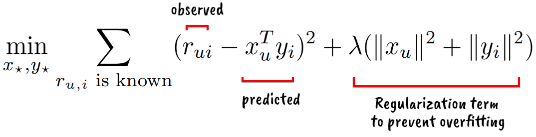
Parameters in the above equation are often learned through stochastic gradient descent.

Work done by Hu et. al divides raw observation $r_{ui}$ into two separate magnitudes with distinct interpretations: preference ($p_{ui}$) and confidence levels ($c_{ui}$).

Hu et. al.⁵ in their seminal paper (Winner of the 2017 IEEE ICDM 10-Year Highest-Impact Paper Award) described an implicit feedback based factorization model idea that gained a lot of popularity. First, they formalized the notion of preference and confidence. Preference $p_{ui}$ is indicated using a binary variable that is 1 for all non-zero and positive $r_{ui}$ values, and is 0 otherwise (when u never consumed i). $p_{ui} = \begin{cases} 1 & r_{ui}>0\ 0 & r_{ui}=0 \end{cases}$ $r_{ui}$ indicates the observations for user actions, for example $r_{ui}$ = 0.7 could indicate that the user u watched 70% of the movie i. If $r_{ui}$ grows, so does our confidence that the user indeed likes the item. Hence the confidence $c_{ui}$ in observing $p_{ui}$ is defined as $1 + \alpha r_{ui}$. This varying level of confidence gracefully handles the noisy implicit feedback issues described previously. Also, the missing values ($p_{ui} = 0$) will have low corresponding confidence.

Similar to the least-squares model for explicit feedback, our goal is to find a vector $x_{u}$ (user factor) for each user u and vector $y_{i}$ (item factor) for each item i that will factor respective user and item preferences. In other words, preferences are assumed to be the inner products: $p_{ui} = x_{u}^{T}y_{i}$. Hence the cost function becomes:

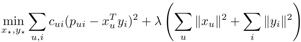
Note that the cost function now contains $m \times n$ terms where m and n are the dimensions of the rating matrix. As this number can easily reach a few billion, the author proposed a clever modification to the alternating least squares method (as opposed to using stochastic gradient descent). The algorithm alternates between re-computing user factors and item factors and each step is guaranteed to lower the value of the cost function. Basically $x_{u}$ can be minimized to: $x_{u} = (Y^{T} C^{u}Y + \lambda I)^{-1} Y^{T} C^{u} p(u)$, which can be further sped up by computing $Y^{T} C^{u}Y$ as $Y^{T}Y + Y^{T}(C^{u}-I)Y$. Similar we calculate $y_{i}$ as $(X^{T} C^{i}X + \lambda I)^{-1} X^{T} C^{i} p(i)$. A slight modification to this calculation also allows for explainable recommendations. Refer to their paper for further details⁵.

Implementing Implicit Feedback Recommender in Python

To implement a recommender based on the above idea, we will use the Last.fm 360K dataset ⁶, and the Python implementation based on Ben Frederickson’s implicit Python package⁷.

  1
  2
  3
  4
  5
  6
  7
  8
  9
 10
 11
 12
 13
 14
 15
 16
 17
 18
 19
 20
 21
 22
 23
 24
 25
 26
 27
 28
 29
 30
 31
 32
 33
 34
 35
 36
 37
 38
 39
 40
 41
 42
 43
 44
 45
 46
 47
 48
 49
 50
 51
 52
 53
 54
 55
 56
 57
 58
 59
 60
 61
 62
 63
 64
 65
 66
 67
 68
 69
 70
 71
 72
 73
 74
 75
 76
 77
 78
 79
 80
 81
 82
 83
 84
 85
 86
 87
 88
 89
 90
 91
 92
 93
 94
 95
 96
 97
 98
 99
100
101
102
103
104
105
106
107
108
109
110
111
112
113
114
115

import numpy as np
import pandas as pd

from numpy import bincount, log, log1p
from scipy.sparse import coo_matrix, linalg

class ImplicitCF:
    def __init__(self):
        self.df = pd.read_csv("lastfm-dataset-360K/usersha1-artmbid-artname-plays.tsv", sep='\t', header=None, names=['user', 'artist', 'plays'], usecols=[0,2,3])
        self.df['user'] = self.df['user'].astype("category")
        self.df['artist'] = self.df['artist'].astype("category")
        self.df.dropna(inplace=True)
        
        self.plays = coo_matrix((self.df['plays'].astype(float),
                                  (self.df['artist'].cat.codes,
                                  self.df['user'].cat.codes)))
    
    def _bm25_weight(self, X, K1=100, B=0.8):
        """Weighs each row of a sparse matrix X  by BM25 weighting"""
        # calculate idf per term (user)
        X = coo_matrix(X)
        N = float(X.shape[0])
        idf = log(N) - log1p(bincount(X.col))
        # calculate length_norm per document (artist)
        row_sums = np.ravel(X.sum(axis=1))
        average_length = row_sums.mean()
        length_norm = (1.0 - B) + B * row_sums / average_length
        # weight matrix rows by bm25
        X.data = X.data * (K1 + 1.0) / (K1 * length_norm[X.row] + X.data) * idf[X.col]
        return X
    
    def _alternating_least_squares(self, Cui, factors, regularization, iterations=20):
        artists, users = Cui.shape

        X = np.random.rand(artists, factors) * 0.01
        Y = np.random.rand(users, factors) * 0.01

        Ciu = Cui.T.tocsr()
        for iteration in range(iterations):
            self._least_squares(Cui, X, Y, regularization)
            self._least_squares(Ciu, Y, X, regularization)

        return X, Y

    def _least_squares(self, Cui, X, Y, regularization):
        artists, factors = X.shape
        YtY = Y.T.dot(Y)

        for u in range(artists):
            # accumulate YtCuY + regularization * I in A
            A = YtY + regularization * np.eye(factors)

            # accumulate YtCuPu in b
            b = np.zeros(factors)

            for i in Cui[u,:].indices:
                confidence = Cui[u,i]
                factor = Y[i]
                A += (confidence - 1) * np.outer(factor, factor)
                b += confidence * factor

            # Xu = (YtCuY + regularization * I)^-1 (YtCuPu)
            X[u] = np.linalg.solve(A, b)
    
    def factorize(self):
        artist_factor, user_factor = self._alternating_least_squares(self._bm25_weight(self.plays).tocsr(), 50, 1, 10)
        return artist_factor, user_factor
    
    def init_predict(self, x_factors):
        # fully normalize factors, so can compare with only the dot product
        norms = np.linalg.norm(x_factors, axis=-1)
        self.factors = x_factors / norms[:, np.newaxis]
    
    def get_related(self, x_id, N=5):
        scores = self.factors.dot(self.factors[x_id])
        best = np.argpartition(scores, -N)[-N:]
        print("Recommendations:")
        for _id, score in sorted(zip(best, scores[best]), key=lambda x: -x[1]):
            print(f"artist id: {_id}, artist_name: {self.df.artist[_id]} score: {score:.5f}")
			
cf_object = ImplicitCF()
print(cf_object.df.head())
#                                       user                artist  plays
#0  00000c289a1829a808ac09c00daf10bc3c4e223b       betty blowtorch   2137
#1  00000c289a1829a808ac09c00daf10bc3c4e223b             die Ärzte   1099
#2  00000c289a1829a808ac09c00daf10bc3c4e223b     melissa etheridge    897
#3  00000c289a1829a808ac09c00daf10bc3c4e223b             elvenking    717
#4  00000c289a1829a808ac09c00daf10bc3c4e223b  juliette & the licks    706
print(cf_object.df.user.nunique()) # 358868
print(cf_object.df.artist.nunique()) # 292364
print(cf_object.df.plays.describe())
#count    1.753565e+07
#mean     2.151932e+02
#std      6.144815e+02
#min      0.000000e+00
#25%      3.500000e+01
#50%      9.400000e+01
#75%      2.240000e+02
#max      4.191570e+05
#Name: plays, dtype: float64
print(cf_object.plays.shape) # (292364, 358868)

artist_factor, user_factor = cf_object.factorize()
print(artist_factor.shape) # (292364, 50)
print(user_factor.shape) # (358868, 50)

cf_object.init_predict(artist_factor)
print(cf_object.factors.shape) # (292364, 50)
cf_object.get_related(2170)
#Recommendations:
#artist id: 2170, artist_name: maroon 5 score: 1.00000
#artist id: 170436, artist_name: vilma palma e vampiros score: 1.00000
#artist id: 257, artist_name: the beatles score: 1.00000
#artist id: 24297, artist_name: dizzee rascal score: 0.77604
#artist id: 257575, artist_name: the velvet underground score: 0.71697

Code is also available on this GitHub Gist.

Summary

In this article, I discussed defining characteristics of explicit and implicit feedback along with their respective shortcomings. Next, I went over one of the most popular research on a factor model which is specially tailored for implicit feedback recommenders. We also implemented factorization-based recommender systems in Python for both explicit and implicit datasets.

References