Statistical vs Machine Learning vs Deep Learning Modeling for Time Series Forecasting

Over recent decades, Machine Learning (ML) and, its subdomain, Deep Learning (DL) based algorithms have achieved remarkable success in various areas, such as image processing, natural language understanding, and speech recognition. However, ML algorithms haven’t quite had the same widely known and unquestionable superiority when it comes to forecasting applications in the time series domain. While ML algorithms have to overcome the challenges in modeling the non-i.i.d. nature of data inherent in the time series domain, statistical models excel in this setting and provide explicit means to model time series structural elements, such as trend and seasonality.

In this article, we will do a deep dive into literature and recent time series competitions to do a multifaceted comparison between Statistical, Machine Learning, and Deep Learning methods for time series forecasting.

Note: This is a long-form article. If you need a TL;DR, feel free to skip to the last section named Takeaways.

What’s the difference between Statistical and Machine Learning forecasting models?

Before continuing, we should define what “statistical” and “machine learning” models are in the context of forecasting. This distinction is not always trivial because a majority of machine learning algorithms are maximum likelihood estimators meaning that they are statistical in nature. Similarly, traditional statistical models, such as autoregressive models, can be specified as linear regression on lags of the series, and linear regression is mostly considered a machine learning algorithm. So to distinguish between the two, we will use the following definition proposed by various researchers ¹².

A statistical model prescribes the data-generating process, for example, an autoregressive (AR) model only looks at the relationship between lags of a series and its future values. Whereas a machine learning model learns this relationship thus being more generic, for example, a neural network creates its own features using non-linear combinations of its inputs. ML methods, in contrast to statistical ones, are also more data-hungry. While the completely non-linear and assumption-free estimation of ML forecasts (e.g., in terms of trend and seasonality) let the data speak for themselves, it also demands a large volume of data for effectively capturing the dynamics and interconnections of the data. Moreover, many statistical methods have developed excellent heuristics that allow even novices to create reasonable models with a few function calls, determining a good approach for ML modeling is more experimental³.

Comparisons based on the forecasting literature

“Statistical and Machine Learning forecasting methods: Concerns and ways forward” by Makridakis et al.

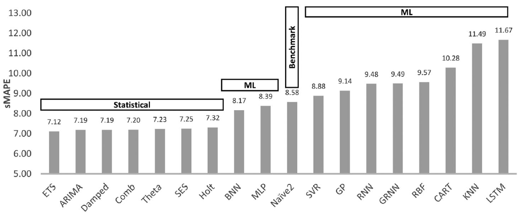
One of the earliest and most popular empirical studies that compared Statistical and ML methods was done by Makridakis et al ⁴. In their 2018 paper, they used a set of 1045 monthly (univariate) time series sampled from the dataset used in the M3 competition to evaluate performances of 8 traditional statistical (Seasonal Random Walk, SES, Holt & Damped Exponential Smoothing, Comb: average of SES, Holt, and Damped, Theta, ARIMA, and ETS) and 10 ML methods (MLP, BNN, RBF, GRNN, KNN, CART, SVR, GP, RNN, and LSTM) on multi-step ahead forecasting task.

To generate multi-horizon forecasts from ML models, they considered three approaches: iterative, multi-node output, multi-network forecasting, and for preprocessing the input, they considered detrending, deseasonalizing, box-cox power transformation, a combination of the three, as well as directly using the original data. They also considered using mean, median, or mode over the outputs of multiple models trained with different hyperparameter initializations and reported the results from the most appropriate alternatives. The following figure shows the overall sMAPE (symmetric Mean Absolute Percentage Error) values averaged over 18 one-step-ahead forecasts for all the models they considered. Similar conclusions were drawn for the case of multi-step-ahead forecasts.

Summary

As seen above, the six most accurate methods were statistical. Even the Naïve 2 (seasonal random walk) baseline was shown to be more accurate than half of the ML methods. Through additional experiments, they also showed that the ML models, specially LSTMs, overfitted the data during training but had a worse performance during the testing phase.

Additional Notes

• ML methods are computationally more demanding, and methods like deseasonalizing the data, utilizing simpler models, and using principled approaches to turning hyperparameters can help in reducing this cost.
• Using a sliding window approach gives as much information as possible about future values and also reduces the uncertainty in forecasting.

“Statistical, machine learning and deep learning forecasting methods: Comparisons and ways forward” by Makridakis et al.

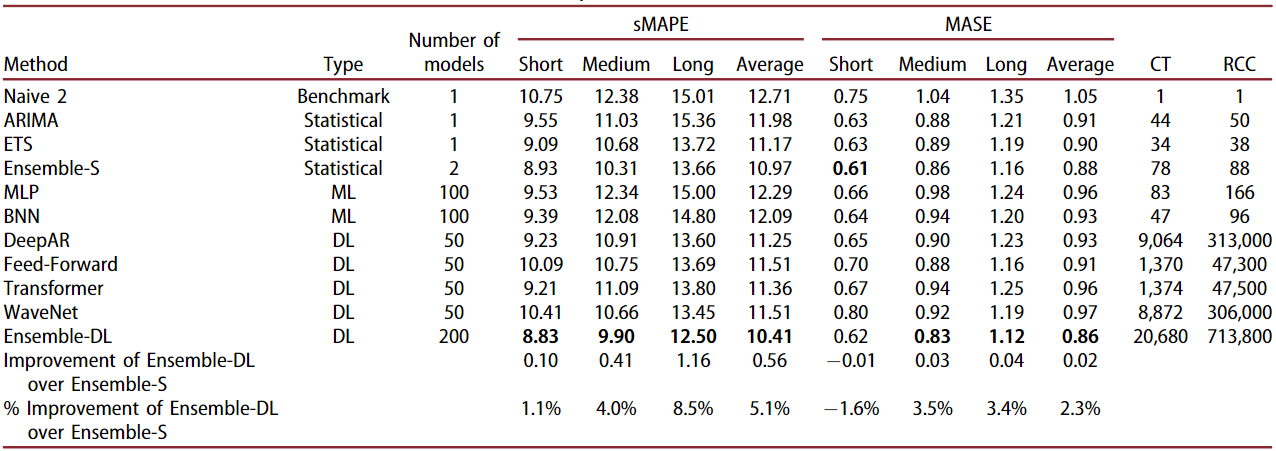
In 2022, the authors of the above paper followed up with another study and added more modern deep learning networks in this comparison ⁵. For statistical models, they used the top-2 performing algorithms from the earlier study: ETS and ARIMA, and an ensemble of the two: Ensemble-S. Similarly, they used top-2 performing ML algorithms: MLP and BNN. Next, they used four modern deep learning algorithms: DeepAR, Feed-forward, Transformer, WaveNet, and an ensemble of the four: Ensemble-DL. The following table shows the sMAPE and MASE accuracy metrics for all of these methods tested on the same 1045 M3 series data using the respective optimal hyperparameters found during experimentation. The computational time (CT), i.e., the time (measured in minutes) required by the methods for training and predicting, as well as the relative computational complexity (RCC) of the methods, i.e., the number of floating point operations required by the methods for inference when compared to the Naive 2, is also reported.

Summary of results at different forecasting horizons

Their experiment shows that ETS and ARIMA are still more accurate on average than the ML methods and many of the individual DL methods across all forecasting horizons (short: 1-6, medium: 7-12, long: 13-18). Both ensembles are more accurate than any of the individual models. Ensemble-DL performed 2-5% better than Ensemble-S overall, but Ensemble-S performed best on MASE on short-term forecasts. ML methods also performed better than DL methods and their ensemble on short-term forecast periods. Long-term forecasts tend to be less accurate than short-term ones for all methods.

Through a separate set of methods, the authors show that when models are optimized based on their one-step-ahead forecasting accuracy, their forecasts will be relatively more accurate for short-term forecasts compared to models that are optimized based on their multi-step-ahead forecasting accuracy, and vice versa. Typically, statistical forecasting methods are optimized in terms of parameters so that the one-step-ahead forecast error is minimized, for example, ETS and ARIMA are parameterized with the objective to minimize the in-sample mean squared error of their forecasts. Similarly, MLP and BNN are parameterized with the objective to produce accurate multi-step-ahead forecasts in a recursive fashion.

Extending to all 3,003 time series of the M3 dataset

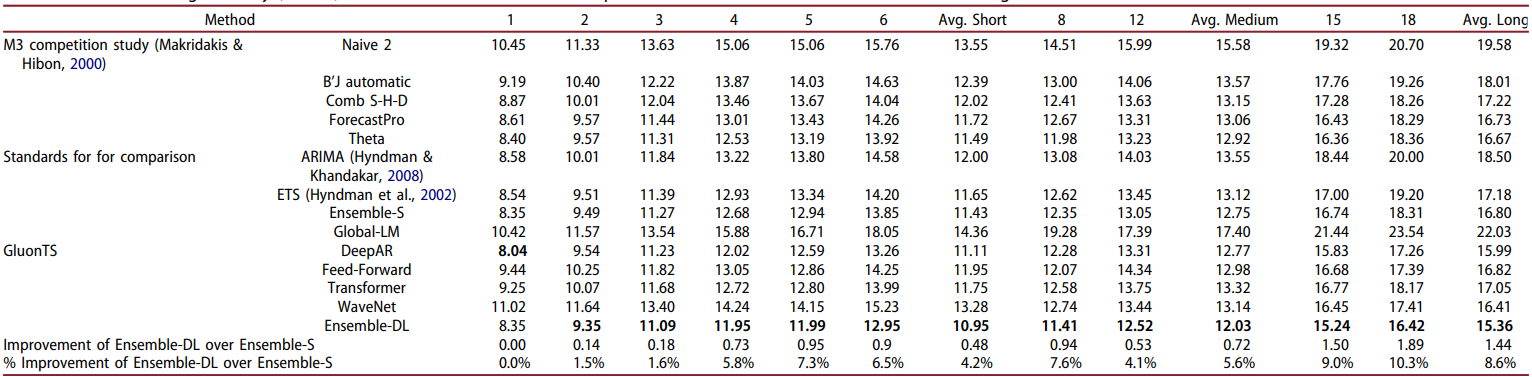
Further expanding their work, the authors considered all of the 3,003 time series of the M3 dataset for the next experiment. The following table shows the resulting sMAPE accuracy both per data frequency and total. The table also shows the reported results from a variety of forecasting methods originally submitted in the M3 competition.

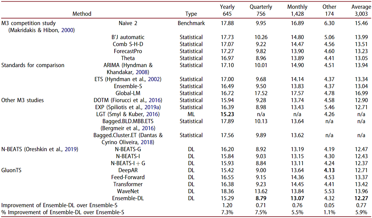
Ensemble-DL continues to be the most accurate forecasting approach overall. DL ensemble was outperformed by a small margin by the LGT model (discussed later) on yearly data, and DeepAR performed better on the data labeled as “Other” (no frequency information available). The Ensemble-DL improvement over Ensemble-S decreases as the data frequency is increased. Ensemble-DL performance is very similar to the N-BEATS method with N-BEATS performing better than Ensemble-DL for the “Other” series.

Balancing the comparison among ensembles

Note that in the above discussion, Ensemble-S only used 2 models while Ensemble-DL had 4. To make a fair comparison, the authors also evaluated the DL models in pairs and found that all of the pairwise DL models performed better than Ensemble-S from 0.4-6.1%.

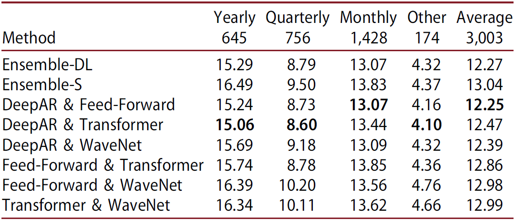
Interestingly, ensembles that involve DeepAR, i.e., the most accurate individual DL model, consistently outperform the rest, while ensembles that involve WaveNet, i.e., the least accurate individual DL model, sometimes deteriorate forecasting performance. Also, the accuracy of Ensemble-DL is comparable to that of the best pairwise ensemble.

Results at different forecasting horizons using all of the M3 data

When examined on various forecasting horizons, with the exception of DeepAR, the individual DL models are less accurate than the best performing statistical one for short and medium horizons, with the differences becoming smaller however as the forecasting horizon increases. For example, Theta is more accurate than the Feed-Forward, Transformer, and WaveNet models for short and medium-term forecasts, and it it also better than Feed-Forward and Transformer models for long-term forecasts. Both Ensemble-S and Ensemble-DL provided more accurate results than those of their constituent methods. However, Ensemble-DL is at least as accurate or superior to Ensemble-S when the complete M3 data set is considered, across all horizons.

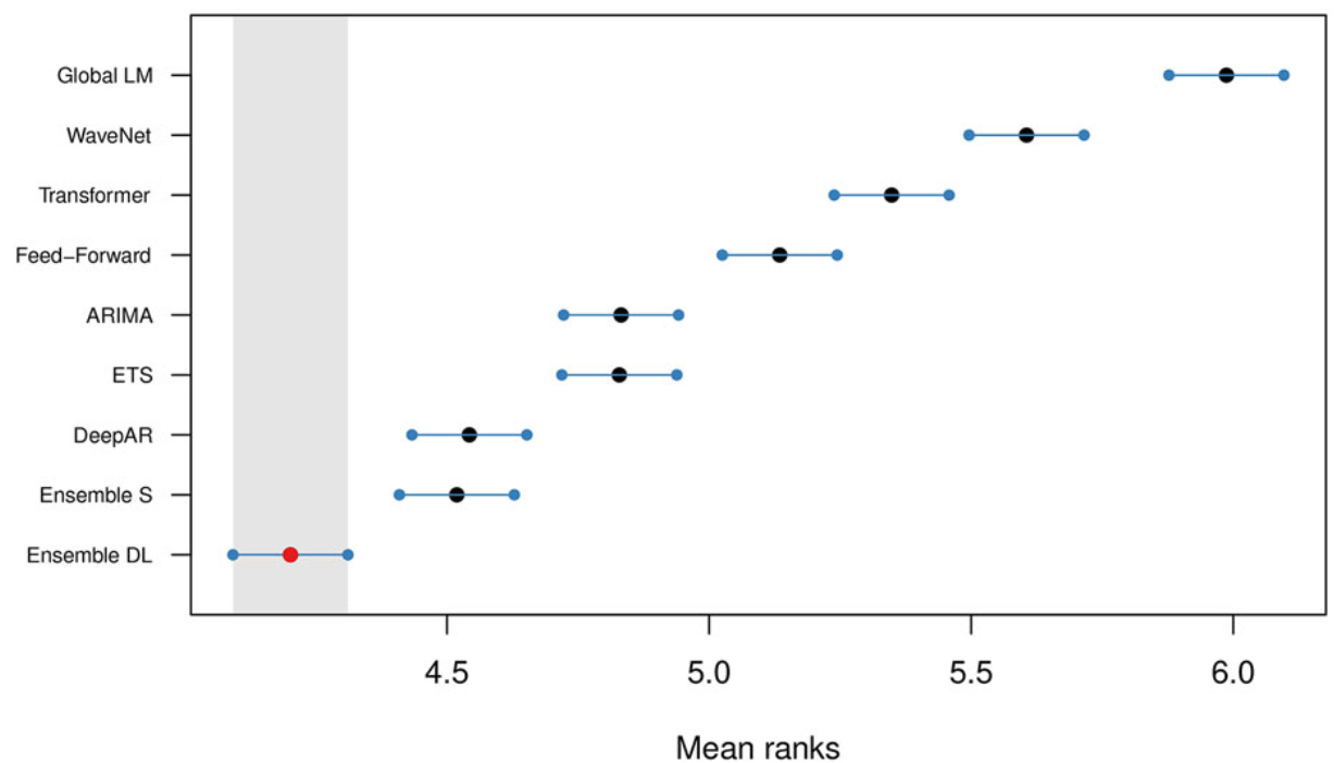
Comparison using the MCB method

When ranked using MCB (Multiple comparisons with the best)⁶ method with 95% confidence intervals, we find that Ensemble-DL is significantly more accurate than the rest of the forecasting methods considered in this study, including the DL models it consists of. On a second level, Ensemble-S provides significantly more accurate forecasts than the contributing ETS and ARIMA models. Overall, the power of ensembling is once again confirmed. Finally, despite the dominance of Ensemble-DL, only DeepAR, among all individual DL methods, produces significantly more accurate forecasts than those of the top-performing statistical methods.

Summary

• In this study, DL models produced more accurate forecasts (up to 6% improvements) than statistical and ML ones, especially for longer forecasting horizons.
• Combinations of DL models perform better than most standard models, both statistical and ML, especially in the case of monthly series and long-term forecasts. However, these improvements come at the cost of significantly increased computational time.

Additional Notes

• The authors recommend the utilization of the series index for data sets that contain a limited number of series and no additional series-specific information. By using the index as an additional feature, models are better poised to identify series-specific behaviors.
• In 2019, the authors of the N-BEATS paper (Oreshkin et al.⁷) did a similar experiment that showed ensembles of multiple DL models achieved more accurate forecasts than standard statistical methods on the M3 competition data. However, the individual DL models used for constructing the ensembles were relatively inaccurate.

“Statistical vs Deep Learning forecasting methods” by Statsforecast

In the paper above, the authors concluded that “We find that combinations of DL models perform better than most standard models, both statistical and ML, especially for the case of monthly series and long-term forecasts.” However, a recent experiment conducted by the authors of the Statsforecast library challenged this deduction by using a more powerful statistical ensemble⁸. They combined four statistical models: AutoARIMA, ETS, CES, and DynamicOptimizedTheta (same as their 6th place winning entry in the M4 competition) and shared sMAPE results on the same M3 data.

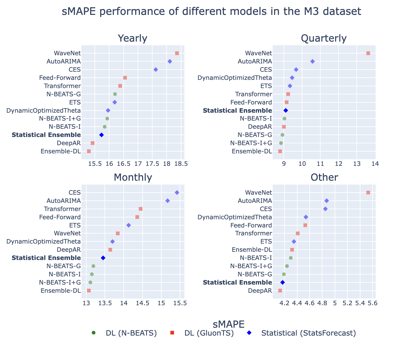
As shown above, their statistical ensemble is consistently better than the Transformer, Wavenet, and Feed-Forward models. The following table summarizes their sMAPE results along with associated costs.

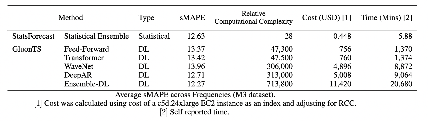
Their statistical ensemble outperforms most individual deep-learning models with average SMAPE results similar to DeepAR but with computational savings of 99%.

Summary

The authors conclude that “deep-learning ensembles outperform statistical ensembles just by 0.36 points in SMAPE. However, the DL ensemble takes more than 14 days to run and costs around USD 11,000, while the statistical ensemble takes 6 minutes to run and costs $0.5c.”.

Additional Notes

In another recent experiment, the authors of Statsforecast compared their statistical ensemble against Amazon Forecast ⁹. Amazon Forecast is a time-series forecasting service on AWS that includes algorithms ranging from commonly known statistical models like ARIMA to complex algorithms like CNN-QR, DeepAR+, etc. They showed that Amazon Forecast’s AutoML was 60% less accurate and 669 times more expensive than running their statistical alternative.

Are there any unique time series characteristics for which some methods perform better than others?

Are there certain methods that can be expected to work reasonably well with data from certain data domains?

We can define a time series in terms of its characteristics such as forecastability (aka spectral entropy), the strength of trend and seasonality, etc. Montero-Manso et al ¹⁰ utilized 42 such features in their runner-up model in the M4 competition. In Makridakis et al.⁵ authors used 5 out 6 features recommended by Kang et al ⁶ for the M3 dataset. The features were: Spectral Entropy, Strength of Trend, Strength of Seasonality, Linearity, and Stability. The sMAPE results for the statistical and deep ensembles were then correlated with these features using a Multiple Linear Regression (MLR).

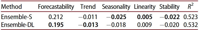
We can see that the Ensemble-DL is generally more effective in handling noisy and trended series, in contrast to Ensemble-S which provides more accurate forecasts for seasonal data, as well as for series that are stable or linear. Similarly, other works show that some methods can be expected to perform better when the time series exhibits certain features like intermittency, lumpiness, or smoothness². Also, sparsity in data might make ML models less effective³.

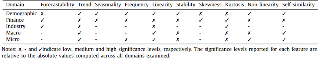
Additionally, research work done by Spiliotis et al.¹¹ shows that certain features are dominant in time series data from the domains in the M4 dataset. This information can provide relevant criteria for model selection. For example, since the following table shows that the financial data tend to be noisy, untrended, skewed, and not seasonal, the Theta method could potentially be utilized to boost the forecasting performance. Accordingly, ETS and ARIMA could be powerful solutions for extrapolating demographic data that are characterized by strong seasonality, trend, and linearity. Additionally, a study of M5 contest submissions shows that the ML methods have entered the mainstream of forecasting applications, at least in the area of retail sales forecasting¹².

Do some models tend to work better with high-dimensional data?

Why do statistical models work better than ML models for small datasets?

Is it better to train a model over multiple time series rather than training it per series?

The author of “Machine learning in M4: What makes a good unstructured model?” paper ³ puts forward an excellent theory in order to explain why ML models tend to work better with high-dimensional data. Kang et al.¹³ showed in their work that certain combinations of time series features may not be possible. Due to their structured nature, statistical models define the class of manifold before the data are observed, which allows the manifold to be defined by a smaller amount of data. However, this comes with a drawback that if the data do not match that class of manifold, the model can never be accurately fitted to it. On the other hand, ML models learn the manifold by observing the data. This creates a more flexible model that can fit more types of relationships but needs more data to define the space.

Another important observation is that Cross-Learning i.e. a single model learning across many related series simultaneously, as opposed to learning in a series-by-series fashion, can enhance forecasting performance. Modeling many series with similar properties is likely to generate a more densely populated, and thus better defined, manifold that is preferred over search spaces with data sparsity. Data normalization used by ML models (as opposed to decomposition-based preprocessing methods used by statistical methods) and rolling-origin cross-validation steps also help in densely populating the same manifold space.

Comparisons based on forecasting competitions

Learnings from the M3 competition

The M3 forecasting competition was held in 2002 and the winner used the Theta method. V. Assimakopoulos and K. Nikolopoulos proposed this method as a decompositional approach to forecasting ¹⁴. Rob Hyndman et al. later simplified the Theta method and showed that we can use ETS with a drift term to get equivalent results to the original Theta method, which is what is adapted into most of the implementations of the method that exist today ¹⁵.

In “Extending to all 3,003 time series of M3 dataset” section, we also saw a few other methods that have since outperformed the Theta method for M3 data. Specifically, the LGT model that was built on the theme of using a statistical algorithm (ETS) for preprocessing followed by an LSTM-based neural network ¹⁶ performed the best on yearly forecast horizon (as measured by sMAPE). The study we discussed also found out that statistical models are better suited for short-term forecasts, while DL ones are better at capturing the long-term characteristics of the data. So it could be beneficial to combine statistical or ML models with DL ones depending on the time horizon of forecasting. LGT model was built on this theme using a statistical algorithm (ETS) for preprocessing followed by an LSTM-based neural network ¹⁶.

Additional Notes

The authors of the LGT paper suggest using categorical variables, like error type, trend type (such as additive, multiplicative), etc. as additional information for improving forecasting accuracy.

Learnings from the M4 competition

The author of the LGT model also authored the winning method of the M4 competition in a similar fashion. The contest-winning model was a truly hybrid forecasting approach that utilized both statistical and ML elements, using cross-learning. This approach used exponential smoothing mixed with a dilated LSTM network¹⁷. The ES formulas enable the method to capture the local components (like per-series seasonality), while LSTM allows it to learn non-linear trends (like NN parameters) and cross-learning. To account for seasonality, the author advocate for incorporating categorical seasonality components (one-hot vector of size 6 appended to time series derived features), and smoothing coefficients into model fitting to allow deseasonalizing of data in the absence of any calendar features like the day of the week or the month number.

Additionally, the second-best M4 method was also based on a cross-learning approach, utilizing an ML algorithm (XGBoost) for selecting the most appropriate weights for combining various statistical methods (Theta, ARIMA, TBATS, etc.) ¹⁰.

Learnings from the M5 competition

Barker’s study ³ pointed out how learning to forecast using multiple time series simultaneously leads to narrower and more densely populated manifolds when the series have a commonality in their origin. The dataset of the M5 competition consisted of more than 30,000 series of daily sales at Walmart. So theoretically we would expect ML models trained in a cross-learning fashion to perform well on this dataset without having to specify additional features. Also, the statistical models that do assume interdependence between the series should perform well. It is worth noting that 48.4% of participating teams could beat the Naïve benchmark, 35.8% could beat the Seasonal Naïve, and only 7.5% of teams could beat the exponential smoothing-based benchmark.

LightGBM, a decision tree-based ML approach, was used by almost all of the top 50 M5 competitors ¹² including the winner, second, fourth, and fifth-positioned teams. The winning submission used an equally weighted combination of various LightGBM models trained on data pooled per store, store-category, and store-department. Runnerup submission used the LightGBM model that was externally adjusted through multipliers according to the forecasts product by an N-BEATS model for the top five aggregation levels of the dataset. The LightGBM models were trained using only some basic features of calendar effects and prices (past unit sales were not considered), and the N-BEATS model was based solely on historical unit sales.

Conclusion

The No-Free-Lunch theorem, proposed for supervised machine learning, tells us that there is never likely to be a single method that fits all situations. Similarly, there is no one time series forecasting method that will always perform best. But the literature suggests a lot of useful learnings that can help us in making more informed decisions when it comes to modeling for time series forecasting. As there are “horses for courses”, there must also be forecasting methods that are more tailored to some types of data and some aggregation levels¹³. The following section lists all of the important takeaways from this article.

Takeaways

• ML methods need more data for better forecasting especially when the series being predicted is non-stationary, displaying seasonality and trend.
• For many years, ML methods have been outperformed by simple, yet robust statistical approaches specifically for domains that involve shorter, non-stationary data, such as business forecasting.
• DL methods can effectively balance learning across multiple forecasting horizons, sacrificing part of their short-term accuracy to ensure adequate performance in the long term.
• Statistical models tend to do well on short-term forecasts, while DL ones are better at capturing the long-term characteristics of the data. So it could be beneficial to combine statistical or ML models with DL ones depending on the time horizon of forecasting.
• Ensemble methods outperform most of the individual statistical and ML models.
• Ensembles of some relatively simple statistical methods like ARIMA, ETS, and Theta, often provide similarly accurate or even more accurate short-term forecasts than the individual DL models and even their ensembles (on rare occasions), but inferior results when medium or long-term forecasts are considered.
• DL ensembles will almost always give better results than Stat ensembles but at a much higher cost and not necessarily a big margin.
• Although the ensembles of multiple DL models lead to more accurate results, depending on the particular characteristics of the series, the additional cost that has to be paid for using a DL model in order to improve forecasting accuracy to a small extent is extensive.
• Some studies suggest that DL methods can lead to greater accuracy improvements, compared to their statistical counterparts, when tasked with forecasting yearly or quarterly series.
• DL ensembles are generally more effective in handling noisy and trended series, in contrast to statistical ensembles that provide more accurate forecasts for seasonal data, as well as for series that are stable or linear. Although DL models are more robust to randomness, seasonality is more effectively modeled by statistical methods.

References