Embedding Collapse in Recommender Systems: Causes, Consequences, and Solutions

Introduction

Representation learning methods are used in modern recommender systems to learn high-quality representations, often without relying on human annotators. These methods represent users and items as low-dimensional representations, approximating the sparse, high-dimensional, user-item interaction matrix. The number of dimensions $d$ in these latent vectors is much smaller than dimension $D$ of the sparse interaction matrix ($d \ll D$). This article describes an issue, called Embedding Collapse, where these learned representations tend to span a subspace of the whole embedding space ($\lt d$), leading to suboptimal solutions.

What is Embedding Collapse?

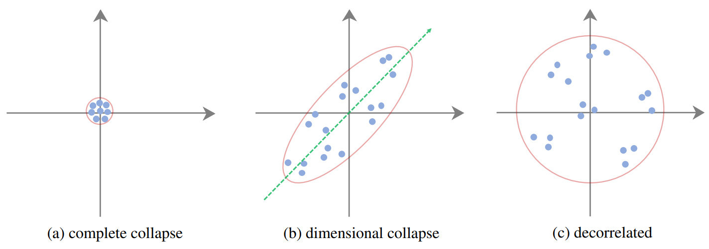
Embedding Collapse refers to a phenomenon in representation learning that can be categorized into the following two types.

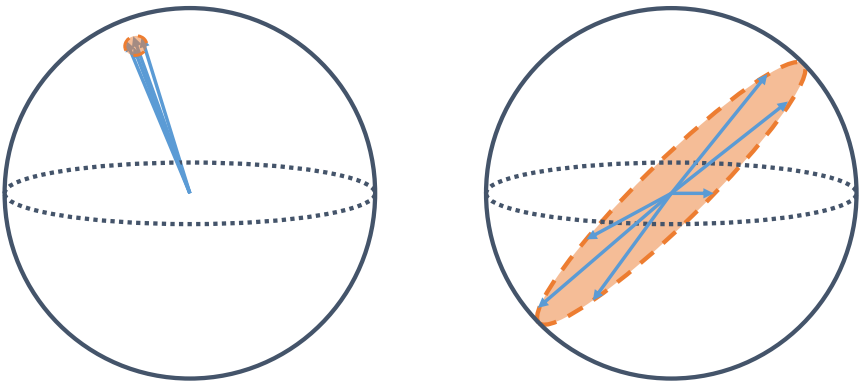
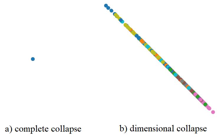
• Complete Collapse, where the representation vectors shrink to a single point in the embedding space (i.e. constant features), meaning that the model creates the same embedding for each input.
• Dimensional Collapse is a less severe, but harder-to-detect collapse pattern where the representation vectors end up occupying a small subspace instead of the full embedding space, i.e. the collapse is along certain dimensions.

Mathematically, the embedding collapse issue can be formulated as $\text{rank}(H^{(L)}) \leq \epsilon$, where $H^{(L)}$ is the embedding when effective rank converges after updating $L$ times, $\epsilon \lt d$, and a smaller $\epsilon$ indicates a more serious collapse. We will revisit effective rank in more detail in the next section.

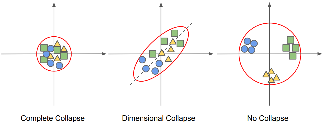
Under ideal conditions, when there is no collapse, representations of items from the same group are closer to each other, while those of items from different groups are as far from each other as possible, as visualized in the next figure ¹.

How Can We Measure Embedding Collapse?

Standard Deviation of the Normalized Embeddings

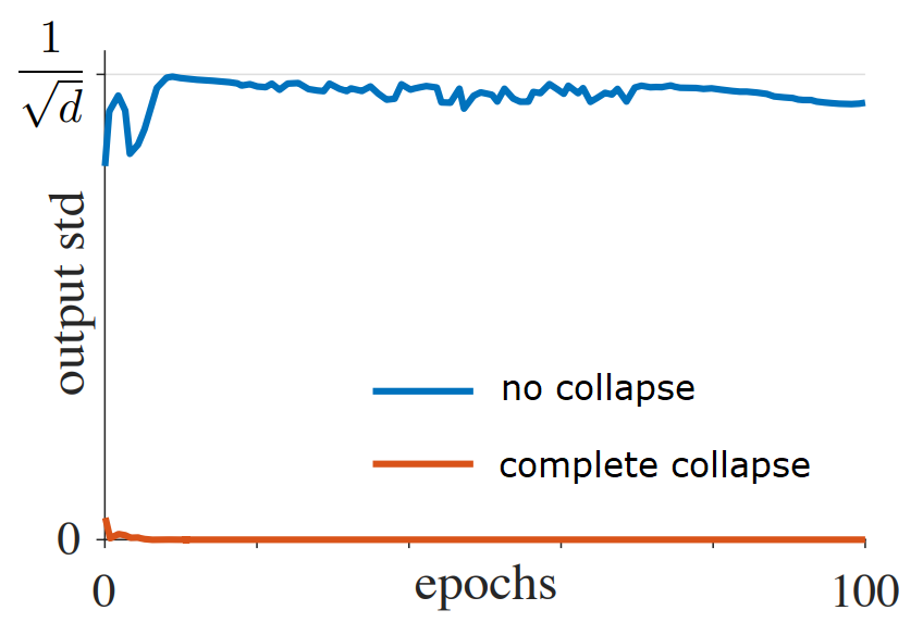
In Chen et al.², Facebook AI researchers looked at the standard deviation of the normalized embeddings to measure embedding collapse. They take the encoder output embedding $z$ and L2-normalize it to get $ \frac{z}{||z||_2} $. Next, the standard deviation of these normalized embeddings is computed across all samples for each dimension in the embedding space. If the embeddings collapse to a constant vector, the standard deviation will be zero for each dimension (i.e., complete collapse). If the embedding follows a zero-mean isotropic Gaussian distribution, the deviation of normalized embedding will be $\frac{1}{\sqrt{d}}$ where $d$ is the embedding dimension. So to use this method, you can track the per-dimension standard deviation averaged over all dimensions during training and compare it against the theoretical $\frac{1}{\sqrt{d}}$ reference for well-distributed embeddings.

Extremely Small Singular Values

In Jing et al.³, researchers at Facebook AI proposed using the Singular Value Decomposition (SVD) of the embedding covariance matrix to quantify embedding collapse. SVD decomposes the covariance matrix $C = U \Sigma V^T$, where $\Sigma$ contains singular values in ascending order. These singular values directly measure the variance explained along different orthogonal directions in the embedding space. A “healthy” embedding distribution should have non-zero singular values across dimensions signifying utilization of all available dimensions. The authors plot the singular values in descending order to visually examine the effective embedding dimensionality. All singular values being close to zero indicates complete collapse, while some singular values being near zero indicates dimensional collapse. The code sample below is adapted from the official GitHub repo of the DirectCLR paper (reference).

def svd_method(embeddings: torch.Tensor) -> None:
    z = torch.nn.functional.normalize(embeddings, dim=1)
    # calculate covariance
    z = z.cpu().detach().numpy()
    z = np.transpose(z)
    c = np.cov(z)
    _, singular_values, _ = np.linalg.svd(c)
    # taking natural log of singular values
    singular_values_log = np.log(singular_values)
    
    plt.plot(range(len(singular_values)), singular_values_log, marker="o", linestyle="-")
    # set other plot params like title, labels, figure size, etc.
    plt.show()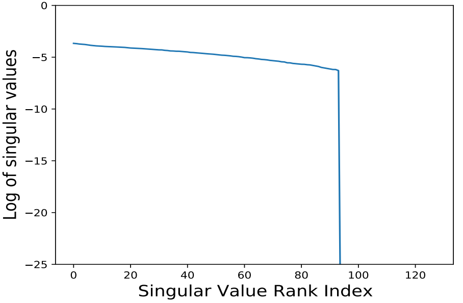

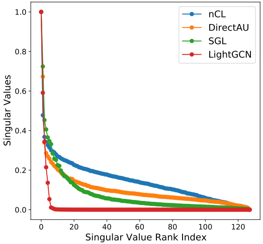
Similarly, Chen et al.¹ calculated singular values of user and item representations’ covariance matrix in sorted order and linearly scaled them to $[0, 1]$. The authors found that all of their tested baseline methods suffered from different levels of dimensional collapse, indicating high redundancy and less information encoded by the learned dimensions.

In Hua et al.⁴, the authors directly visualized the output of the projector layer in 2D projection space to build up intuitions about the reachable collapse patterns. To do this they simply set the output dimension of the projector to 2, and plot visualization like the one shown below.

Information Abundance

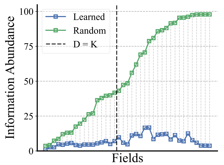
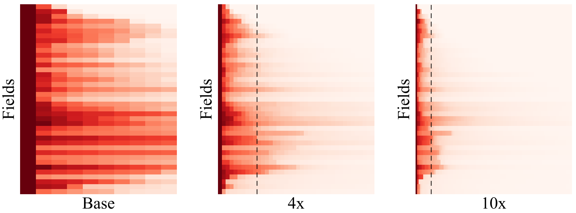
In Guo et al.⁵, researchers at Tsinghua University propose Information Abundance (IA) as a metric to quantify the dimensional collapse of an embedding matrix. It is calculated as the sum of all singular values, divided by the maximum singular value. For an embedding matrix with balanced distribution in the vector space, all singular values will be similar, hence information abundance would be high. On the flip side, if a matrix does not effectively utilize its available dimensions, a certain set of smaller singular values can be compressed, hence the corresponding information abundance value will be small. Mathematically, IA is defined as: $\text{IA}(E) = \frac{\lVert \sigma \rVert_1}{\lVert \sigma \rVert_\infty}$. This formulation is a continuous extension of the concept of matrix rank. A value of 1 for IA indicates complete collapse, while K (i.e. the number of embedding dimensions) indicates no collapse. The authors also use IA to show that the embedding collapse phenomenon is not just a consequence of the cardinality of categorical fields. As shown in the next figure, the learned embeddings of a DCNv2 model on the Criteo dataset have lower IA than random initialization, even in fields where full dimensionality ($D>K$) is theoretically possible. Meaning that the learned embedding matrix is approximately low-rank.

In Pan et al.⁶, the Tencent Ads system also uses IA as a general quantification for collapse. The following code for plotting singular values is adapted from their RecScope GitHub repo (reference).

def recscope_info_plot(embeddings: torch.Tensor) -> None:
    singular_values = torch.SVD(embeddings).S
    singular_values /= singular_values.max()
    # ensure singular values are in 2D format suitable for heatmap
    singular_values_2d = singular_values.unsqueeze(0)
    # create a heatmap (more on it in a next section)
    ax = sns.heatmap(singular_values_2d, cmap="Reds", vmin=0.0, vmax=1.0, annot=False, cbar=True)
    # set plot labels, titles etc.
    plt.show()

Effective Rank

In 2007, Roy et al.⁷ introduced the concept of Effective Rank (erank) as a measure that quantifies how many embeddings a matrix is “effectively” using. It is a real-valued metric (an extension of the integer-valued rank) that is always between 1 and the actual rank. Imagine a 2D space where 90% of the variance is in one direction, while only 10% is in the other. The traditional rank in this case is still 2, whereas the effective rank will be closer to 1, reflecting the domination of one dimension. The effective rank of a matrix $A$ represents the average number of significant dimensions in the range of $A$. To compute erank, singular values of the matrix are normalized into a probability distribution. The entropy of this distribution measures the dimensional balance. High entropy indicates dimensions are being used evenly and hence erank is high. Similarly, uneven dimensional usage will lead to low entropy and low erank.

Mathematically, given the singular values of the embedding matrix $A: \sigma_1 \geq \sigma_2 \geq \cdots \geq \sigma_d \geq 0$, let $p_k = \frac{\sigma_k^2}{\sum_k \sigma_k^2}$, then erank is defined as: $\text{erank}(H) = \exp \left( H(p_1, \cdots, p_d) \right)$, where $H(p_1, \cdots, p_d) = -\sum_k p_k \log p_k$ is the Shannon entropy.

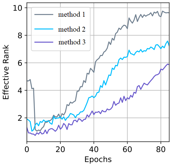
Zhang et al.⁸ used erank as evidence of embedding collapse in contrastive learning-based recommender systems. They tracked the change in erank during training to observe the dimensional diversity.

Peng et al.⁹ also utilized erank in a similar fashion. The following code is adapted from their implementation on GitHub (reference).

def get_erank(embeddings: torch.Tensor) -> float:
    # using numpy svd, as torch.svd was flaky during my experiments
    embeddings_np = embeddings.detach().cpu().numpy()
    values = np.linalg.svd(embeddings_np, full_matrices=False, compute_uv=False)
    # normalize singular values
    values_normalized = values / np.sum(values)
    # calculate entropy
    entropy = -(
        values_normalized * np.nan_to_num(np.log(values_normalized), neginf=0)
    ).sum()
    # calculate erank and convert it to scalar
    erank = np.exp(entropy).item()
    return erank

What Causes Embedding Collapse?

Two-Tower Models

Two-tower (or Dual-encoder) models are heavily used in large-scale recommender systems. The retrieval stage in these industrial systems is usually limited by strict infrastructure constraints, hence the most common choices at this stage include late fusion technique, fixed-sized representations (embeddings), and a dot-product interaction. These models are generally some form of Siamese/dual architecture and often use contrastive learning with negative sampling. Both the user tower and item tower map inputs to a shared embedding space. Refer to this article to learn more about the two-tower models. Jing et al.³ identified two mechanisms that lead to a dimensional collapse in Siamese/contrastive learning method for visual representation learning:

1. Augmentation-driven Collapse: Self-supervised visual representation learning methods aim to learn representations invariant to data augmentations by maximizing the agreement between embedding vectors from different augmentations of the same training instance. The authors show that dimensional collapse occurs when the variance caused by data augmentation exceeds the variance in the original data distribution along certain dimensions. Although data augmentations are more common in Computer Vision, the broader principle still applies to recommenders for any form of input noise/perturbations that exceed natural signal variance, or for models based on sequential masking or multiple views of user behavior.
2. Implicit Regularization: Previous studies have shown that overparametrized neural networks with multiple layers tend to find local minima and can also derive low-rank solutions. The main reason for this is the implicit regularization dynamics of gradient descent causing adjacent weight matrices to align during training. For recommenders that utilize deep neural architectures, user/item embedding layers are followed by multiple dense layers. This tendency toward low-rank solutions could explain why some recommender embeddings don’t utilize the full dimensionality.

Note that the authors also show that directly calculating the distance between two embeddings can also lead to embedding collapse. Hence they utilize a projection matrix upon embeddings before computing the inner product. Chen et al.² also show that models that optimize representation learning only based on the positive pairs tend toward complete collapse solutions where all inputs are mapped to the same constant vector.

Feature-Interaction Based Models

Feature-interaction-based recommender systems, like FM, DeepFM, and DCN, explicitly model interactions between different fields. Categorical fields (such as user id, item id, and item category) are embedded into dense vectors and explicitly interacted with each other through Factorization-Machine-like models. A key aspect of such methods is how the field embeddings interact with each other to capture complex patterns in the data. While these models have had great success in several real-world recommendation systems, recent research suggests that their feature interaction aspect can also cause embedding collapse. Guo et al.⁵ were the first ones to identify this problem through empirical evidence and theoretical analysis, which they called interaction-collapse theory. They present the following two-sided effect of feature interaction modules.

• Feature interactions as a source of collapse: The authors conducted a sub-embedding analysis and showed that the information abundance is co-influenced by the fields it interacts with. And, interacting with a low-information abundance field or matrix will result in collapsed embeddings in general models, even without sub-embeddings as low IA embeddings constrain the IA of other fields. For example, some fields, such as Gender, have very low cardinality and can only span a limited embedding space. When this field interacts with a high-dimensional embedding, it causes the latter to collapse to a lower-dimensional subspace.
• Feature interactions as a necessity: Even though the interaction-collapse theory suggests that feature interaction is the primary reason for the collapse, pair-level feature interaction is a necessary component and cannot be removed. Through empirical tests, the authors show that feature interactions bring domain knowledge of higher-order correlations and help form generalization representations. When feature interaction is restricted, the models tend to fit noise as the embedding size is increased, resulting in reduced generalization.

The authors also empirically show that the limited availability of data does not seem to cause collapse. Information Abundance does not seem to increase or decrease with data size, especially for larger models. And, the embedding collapse phenomenon is “data-amount-agnostic”.

GNN-based Models

Despite their theoretical advantages, GNN architecture-based recommender models, like LightGCN, often underperform simpler models. Recent research suggests that susceptibility to embedding collapse could be the reason behind this. Peng et al.⁹ identify two reasons why GNN-based recommender could suffer from embedding collapse:

• Collapse due to feature interactions: Most GNN-based recommenders like LightGCN ultimately rely on feature interactions, as the iterative message passing/aggregation between nodes is a form of interaction. Based on the interaction-collapse theory presented above, these models are likely to suffer from embedding collapse.
• Collapse due to over-smoothing: In GNN-based models, each layer’s message passing is equivalent to applying a low-pass filter multiple times, i.e. the nodes become increasingly similar/indistinguishable over layers. This causes the loss function to converge faster, which accelerates the embedding collapse. A higher number of layers means even more aggressive filtering and faster collapse. Through experiments, the authors show that LightGCN’s embeddings collapse much faster than Matrix Factorization.

Why is Embedding Collapse bad?

It is important to note that a higher erank, i.e. high-dimensional utilization does not necessarily translate to higher accuracy. Peng et al.⁹ point out that from a spectral perspective, not all dimensions will be equally important to users or items. It is normal for some dimensions to contain more important information than others. So why should you care if all dimensions contribute to the representations?

Reduced Representation Power

Collapsed embeddings tend to occupy a small subspace of the whole embedding space. Generally speaking, this concentration of information in a few dimensions weakens the distinguishability of representations for downstream tasks. Despite having high-dimensional space available, the diversity of learnable information becomes restricted leading to a suboptimal solution. It is particularly problematic for recommender systems where our goal is to learn low-dimensional approximations of the sparse, high-dimensional interaction data.

Learning and Optimization Issues

Hua et al.⁴ observe that with collapsed solutions, gradients become negligible thus compromising learning and utility. It also reduces the model’s generalization ability, as collapse creates a bottleneck preventing learning of complex patterns. This often translates to poor performance on long-tail items.

Barrier to Scaling

Recent research in domains like language modeling has shown that large-scale models with billions of parameters can achieve remarkable performance. However, scaling recommender systems have been challenging. Tencent’s Ads Recommendation team shared that more than 99.99% of parameters in their production model are from feature embeddings⁶. Upon scaling up their recommender systems by increasing embedding dimensions from 64 to 192, they observed no significant performance improvement and even observed performance degradation at times. They found that their embeddings ended up spanning only a lower-dimensional subspace, leading to vast wastage of model capacity as well as reduced ability to capture complex user-item relationships. These findings led them to propose the interaction-collapse theory discussed in the previous section.

Increased Popularity Bias

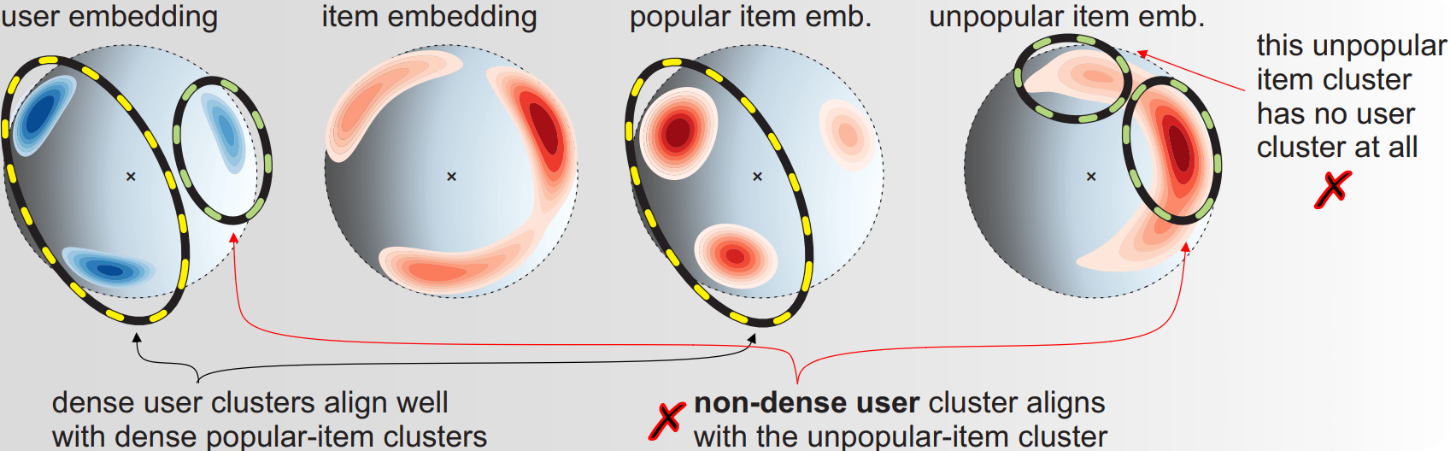
Zhang et al.⁸ found that when embeddings collapse to a lower dimensional space, they tend to cluster towards a few popular items, leading to popularity bias. The authors posit that the dimensionality collapse and popularity bias in collaborative filtering are two sides of the same coin. Most users only interact with a small subset of items in the vast interaction space, hence the popular items already disproportionately influence learning, for example during message passing in Graph Collaborative Filtering (GCF). Embedding collapse further exacerbates this problem. User embeddings collapsing around a few popular item embeddings means that popular items will get recommended more. As shown in the next figure, user and item embedding cluster in just a few regions. Unpopular items get clustered together in one area with sparse user embeddings nearby, meaning that these items rarely get recommended. This creates a “Matthew Effect”, where popular items get more popular, and discovery for niche or long-tail items gets reduced.

How to Handle Embedding Collapse?

Contrastive Learning via Negative Sampling

Contrastive Learning is quite popular in un-/self- supervised learning and several contrastive learning solutions are based on Siamese networks. Contrastive learning via negative sampling is intended to solve the complete collapse issue. By pulling the positive pairs closer and pushing the negative pairs apart in the embedding space, it forces embeddings to spread out to minimize loss. Using larger batch sizes to provide more negative samples has also been shown to be helpful. Negative sampling acts as a high-pass filter and allows high-frequency components (i.e. unique/distinct patterns) to pass through. In recommender systems, it offers a promising solution to address cold-start issues and reduce exposure bias. However, it is not a strong enough deterrent for solving dimensional collapse. In practice, contrastive learning benefits from a large number of negative samples, but increasing the negative sampling ratio can’t alleviate collapse beyond a certain ratio⁹. Also, negative sampling only works with certain loss functions like Bayesian Personalized Ranking (BPR), and Binary Cross-Entropy (BCE).

Non-contrastive Structural Fixes

Hua et al.⁴ connect dimensional collapse with a strong correlation between axes and propose a feature decorrelation approach, i.e. standardizing the covariance matrix in a non-contrastive learning setup. The authors show that the complete collapse pattern is associated with vanishing gradients and it can be addressed by the standard Batch Normalization (BN) that centers and scales activations. While BN standardizes the variance of features, it does not address the string correlation between different feature dimensions. Therefore it cannot prevent dimensional collapse where features become highly correlated. The authors further propose a decorrelated batch normalization (DBN) to help prevent dimensional collapse. Among other non-contrastive solutions, Chen et al.² propose a stop-gradient-based method to prevent collapse.

Multi-Embedding Design

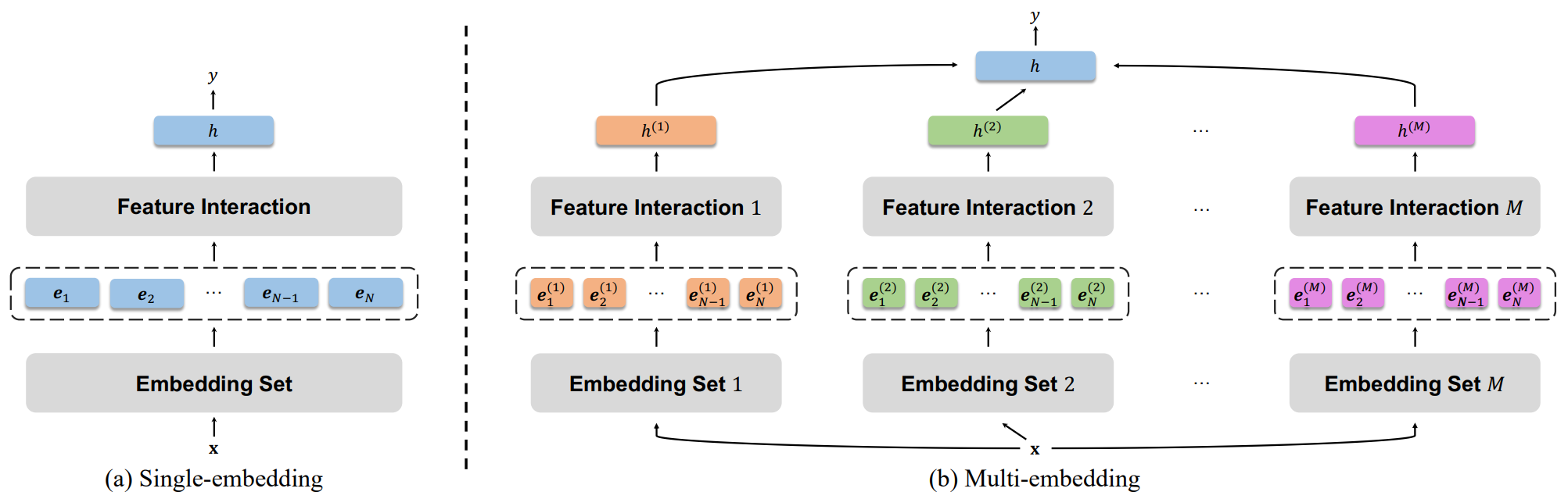
In their interaction-collapse theory for feature-interaction-based recommender systems, Guo et al.⁵ highlighted the need to maintain feature interactions while preventing collapse. They empirically show that suppressing feature interactions may lead to a less collapsed model, but the model also falls into the issue of overfitting and lacking scalability. As a solution, they proposed creating multiple embedding sets instead of increasing the embedding size. Each feature interaction module has its own embedding set, and the output from different independent embedding sets is combined at the end. This separation of field-level interactions helps to learn different interaction patterns jointly and results in embedding sets with large diversity. To prevent the reduction of multiple embedding into a single embedding, a non-linear projection is also added after the interaction. The output projections are averaged to produce the final representation.

Loss Function-based solutions

Wang et al.¹⁰ proposed two-key properties for representation learning that contrastive loss asymptotically optimizes.

• Alignment: Two positive pairs of embeddings should be mapped nearby, and thus be mostly invariant to noise factors.
• Uniformity: Embeddings should be roughly uniformly distributed on the unit hypersphere, preserving as much data as possible.

They provide directly optimizable metrics to quantify and optimize these properties and show that directly optimizing for these two properties leads to representations with comparable or better performance at downstream tasks than contrastive learning.

# bsz : batch size (number of positive pairs)
# d   : latent dim
# x   : Tensor, shape=[bsz, d]
#       latents for one side of positive pairs
# y   : Tensor, shape=[bsz, d]
#       latents for the other side of positive pairs
# lam : hyperparameter balancing the two losses

def lalign(x, y, alpha=2):
	return (x - y).norm(dim=1).pow(alpha).mean()
def lunif(x, t=2):
    sq_pdist = torch.pdist(x, p=2).pow(2)
    return sq_pdist.mul(-t).exp().mean().log()
loss = lalign(x, y) + lam * (lunif(x) + lunif(y)) / 2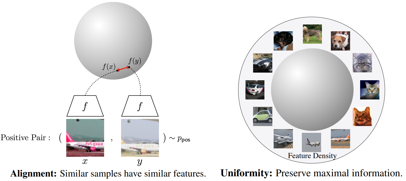

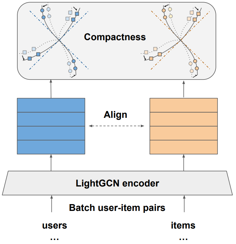
In Chen et al.¹, researchers at Visa build on this work in the recommender systems domain and propose a different balance of geometric properties:

• Alignment uses the same principle and tries to push together representations of positive-related user-item pairs.
• Compactness uses rate-distortion theory to replace the uniformity principle by finding the optimal coding length of user/item embeddings, subject to a given distortion.

The authors propose a method called nCL (non-contrastive learning) that achieves the two properties by maximizing the overall volume of embeddings while minimizing within-cluster volume. For obtaining cluster information they propose a graph topology-based variant and a learned assignments variant.

In Zhang et al.⁸, the authors propose a loss function called LogDet, defined as: $L_{logdet} = tr(ΣU + ΣI) - \log{\det{(ΣUΣI)}}$

where $ΣU$ and $ΣI$ are the covariance matrices for user and item embeddings respectively, $tr$ is the trace operation (sum of diagonal elements), $det$ is the determinant and $log$ is the natural logarithm. If any singular value approaches 0, the log det term approaches negative infinity. This strategy creates an infinite penalty, strictly preventing collapse, whereas previous methods apply a finite penalty, like uniformity loss.

Balancing Embedding Spectrum

Peng et al.⁹ argue that optimizations on observed interactions act as a low-pass filter (making embeddings similar) while negative sampling acts as a high-pass filter (pushing embeddings together), but neither fully solves the collapse. They propose a method called DirectSpec that acts as an “all-pass filter” to balance the spectrum distribution of embeddings, such that all dimensions contribute equally. The authors note that in recommender systems, perfect decorrelation (user/user or item/item) is not the goal. Users who share interests should have similar embeddings, while users with completely different interests should have very different embeddings. Similarly, items that are never liked by the same user should have different embeddings, while items often liked by the same users should have similar embeddings. So observed pairs should be correlated and unobserved pairs should stay irrelevant. So the authors propose an extension to their algorithm called DirectSpec+ that uses self-paced gradients to balance correlation and decorrelation. The authors shared their implementation for the two variants on GitHub (link).

Conclusion

This article provided a deep dive into the embedding collapse phenomenon where the learned representation does not make full use of all dimensions. In a complete collapse pattern, all embeddings trivially collapse to the same point/vector. While dimensional collapse occurs when embeddings only span a low-dimensional subspace of the available space. Interestingly, simply reducing the size of dimensions (for example, 128 → 64) does not solve the collapse problem¹. Collapse reduces expressiveness, wastes model capacity, and leads to issues like popularity bias. We also looked at ways to visualize and quantify the embedding collapse problem and went through several contrastive and non-contrastive solutions for the collapse problem.

References