Skip List Data Structure - Explained!

Why am I writing about Skip Lists?

Skip List is one of those data structures that I have seen briefly mentioned in academic books; but never seen it being used in academic or industrial projects (or in LeetCode questions 🙂 ). However I was pleasantly surprised to see Skip List being one of the major contributors behind Twitter’s recent success in reducing their search indexing latency by more than 90% (absolute). This encouraged me to brush up my understanding of Skip List and also learn from Twitter’s solution.

Why do we need Skip Lists?

I believe it’s easier to understand the concept of Skip Lists by seeing their application. So let’s first build a case for Skip List.

The Problem: Search

Let’s say you have an array of sorted values as shown below, and your task is to find whether a given value exists in the array or not.

Given an array:

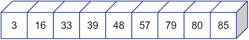
find whether value 57 exists in this array or not

Option 1: Linearly Searching an Array

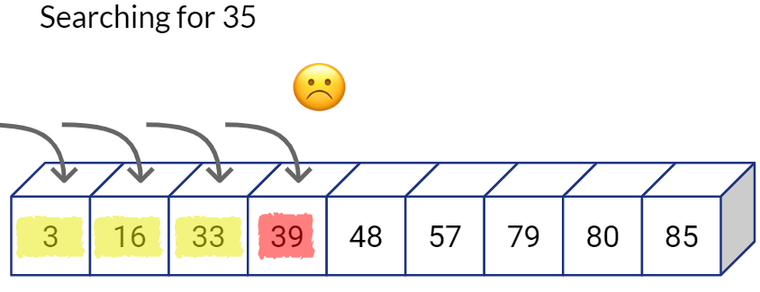
As the name suggests, in linear search you can simply traverse the list from one end to the other and compare each item you see with the target value you’re looking for. You can stop the linear traversal if you find a matching value.

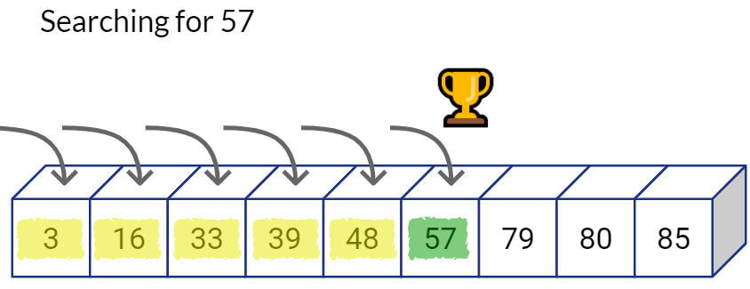
You can stop the search if at any point of time you see an item whose value is bigger than the one you’re looking for.

Option 2: Binary Search on an Array

The binary search concept is simple. Think of how you search for a given word in a dictionary. Say if you are trying to find the word “quirky” in the dictionary, you do not need to linearly read each word in the dictionary one-by-one to know if the word exists in the dictionary. Because you have established that the dictionary has the all of the words in alphabetical sorted order. You can simply flip through the book, notice which word you are at, then either go left or right depending on whether the word starts with a character that comes before or after ‘q’.

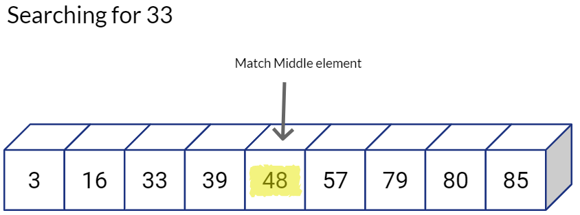
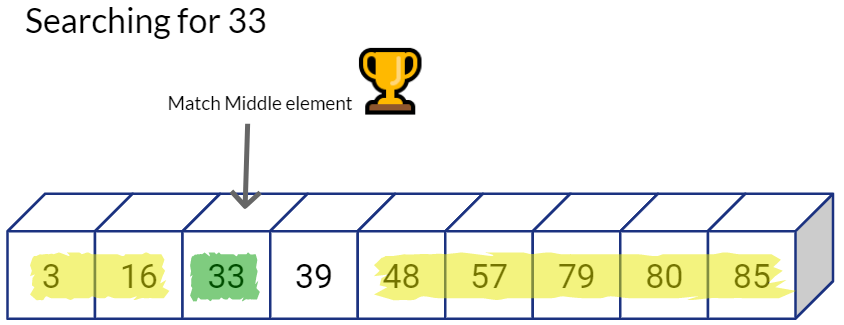
Going back to our example, let’s first check the value at the center of the sequence, if the value matches our target. we can successfully end the search.

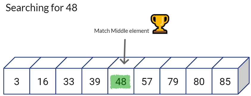
But if it is not the value we are looking for, we will compare the value of the middle position with our target value. If our target value is smaller, we need to look into smaller numbers, so we go towards left and ignore the values on the right.

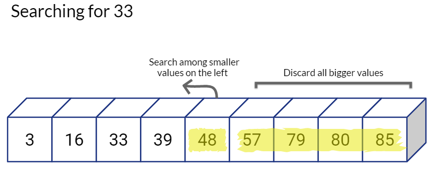
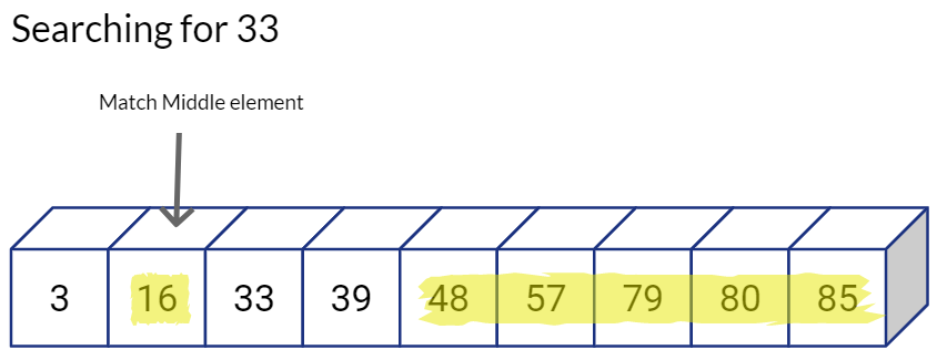
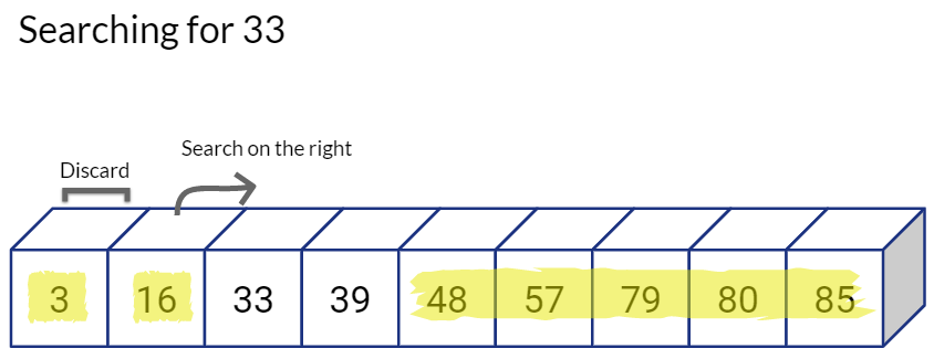
By following this binary search approach have reduced our search space and the required number of comparisons by half. Also, we repeat the same process on the “valid” half, i.e. we directly go the middle value of the left sub-array and see if we have a match, if not, we again decide whether to go left or right, and hence reduce our candidate search space by half again.

This is excellent. Logarithmic time complexity means that our algorithm will scale really well with large number of values being stored in the sequential array.

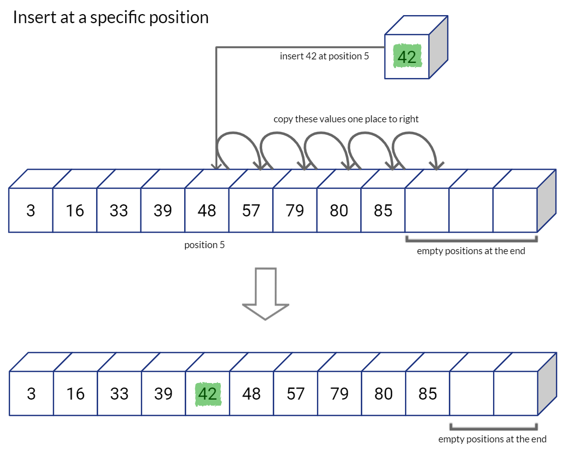
As you can imagine, having extra space on the right of the array would be convenient else you would have to call for dynamic allocation of memory at every insertion and copy over the whole array to newly allocated array memory. List data structure in Python, allocates list in a similar way that leaves capacity at the end of the sequence for future expansion. If we run out of space in the list, Python allocates a new and much larger (double the size, for example) sized list, copies over each value from the old list to new list, and then deletes the old list. (This is why the insertion in a Python list is Amortized O(1) complexity)

Option 3: Linear search with Linked Lists

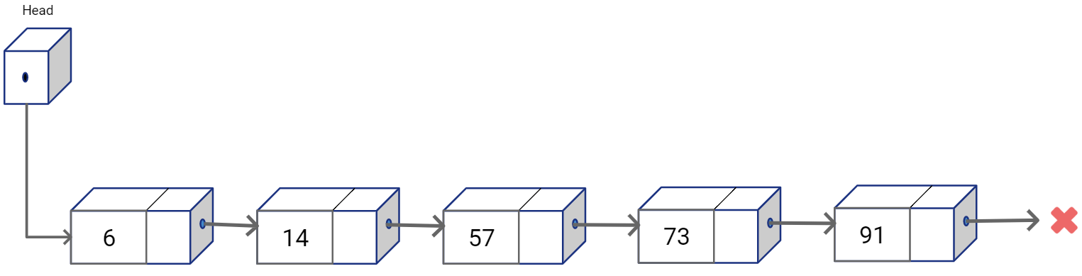
Linked Lists are dynamic data structures that store values in non-contiguous memory blocks (called nodes). Each block refers to the other using memory pointers. These pointers are sort of the links in a chain that define the ordering among the non-contiguous nodes. A Singly Linked list represents a sequential structure where each node maintains a pointer to the element that follows it in the sequence. In linked lists we also maintain additional reference to the list nodes. Head is one such reference which is variable that stores the address for the first element in the list (stores null pointer if the list is empty).

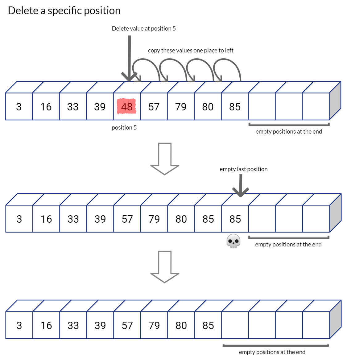
Insertion and deletion at any arbitrary location is straightforward, as you would simply reconnect the links of the nodes previous and next positions from the target position.

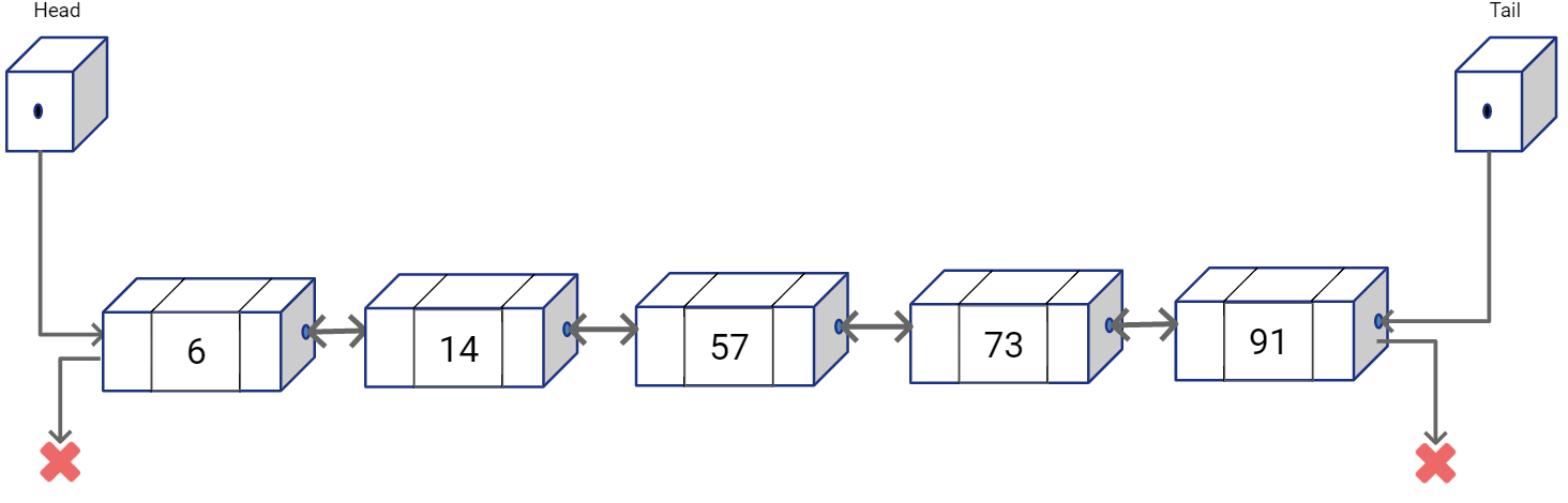
We can also have a Doubly Linked List where each node stores the pointer to the previous as well as the next node in the sequence. A tail reference may also be used to store pointer to the last node in the linked list.

As you would notice, random access in linked lists are not possible. And to find a value in the list, we would simply have to traverse the list from one end, say from the node referred by Head, towards the other end till we find what we are looking for. So, even though you can insert and delete in O(1), you still need the reference to the target location. Finding the target location is again O(n).

With Linked Lists, while we solved the issue of costly insertions and deletions, we haven’t quite found a good solution to quickly access a target value in the list (or find if the value exists).

Wouldn’t it be great if we could have the random access (or something close to it) in the list to simply our find, insert and delete operations? Well this is where Skip List come handy!

Option 4: Pseudo-binary search with Linked Lists [Skip List]

Technical advances have made low latency highly desirable for software applications. How well the underlying algorithm scales to demand can make or break a product. On the other hand, the memory/storage costs is getting cheaper by day. This propels many system designers to make decisions that balance compromises that spend extra money on storage costs, while opting for algorithms with low time complexities. Skip Lists is a good example of one such compromise.

Skip Lists were proposed by WIlliam Pugh in 1989 (read the original paper  here) as a probabilistic alternative to balanced trees. Skip lists are relatively easy to implement, specially when compared to balanced trees like AVL Trees or Red Black Trees. If you have used the Balanced Trees before, you may remember how they are great data structures to maintain relative order of elements in a sequence, while making search operations easy. However, insertions and deletions in Balanced Trees are quite complex as we have the additional task to strictly ensure the tree is balanced at all times.

Skip Lists introduce randomness in by making balancing of the data structure to be probabilistic. While it definitely makes evaluating complexity of the algorithm to be much harder, the insertion, deletion operations become much faster and simpler to implement. The complexities are calculated based on expectation, but they have a high probability, such that we can say with high confidence (but not absolute guarantee) that the run time complexity would be O(log(n)) apart from some specific worst-case scenarios as we would see soon.

Skip Lists - Intuition

Following is the map of New York Subway’s “7” train.

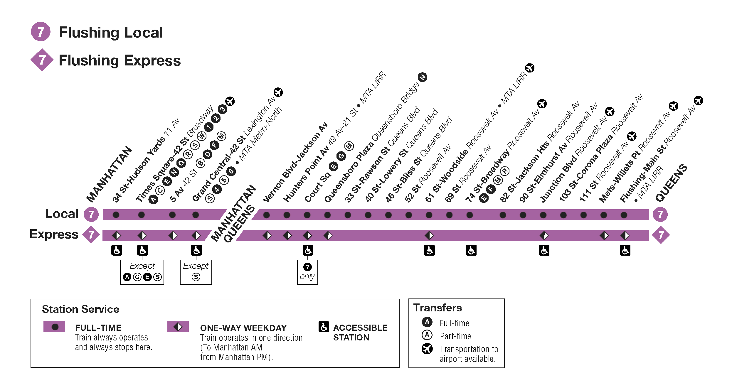
Each point on the horizontal line represents on train stop on a specific street. The line at the top is the local train that has much more number of stops compared to the express line on the below it. Government decides where to put the stops based on factors like nearby facilities, neighborhood, business centers etc. Let’s simplify the above route map and display stations by the street numbers.

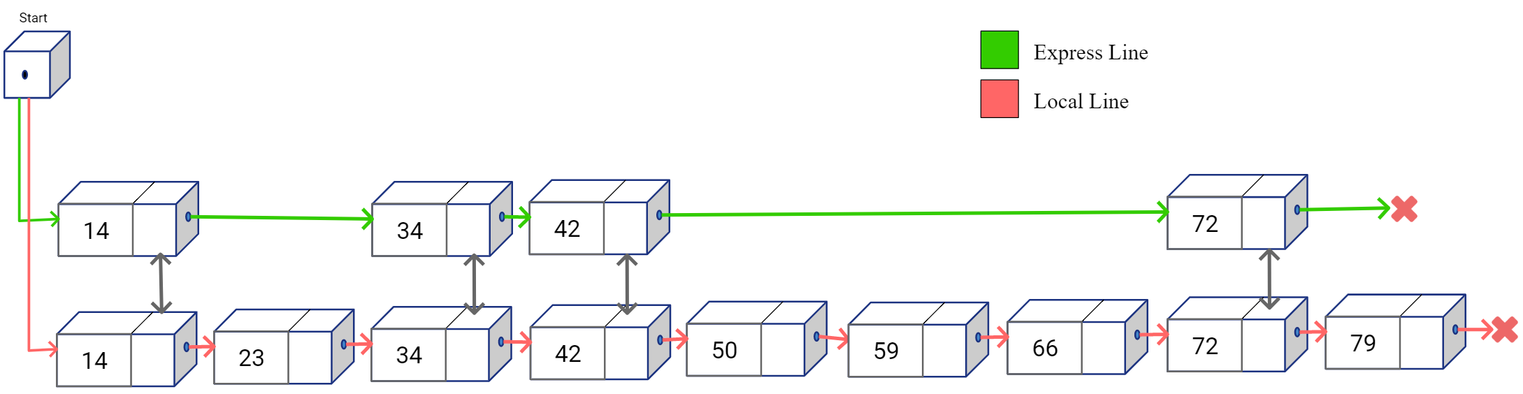
In the simplified map above, the express line is shown at the top and local line is below it. Now if you had this map and you were supposed to travel from stop 14 to stop 59. How would you plan your trip route? For simplicity let’s assume we can’t overshoot, meaning that we can’t go some station to the right and then travel back towards left. You would probably want to take the express line from stop 14 and get down on stop 42. Then take the local train from stop 42 and reach the destination 59 from there, as shown below.

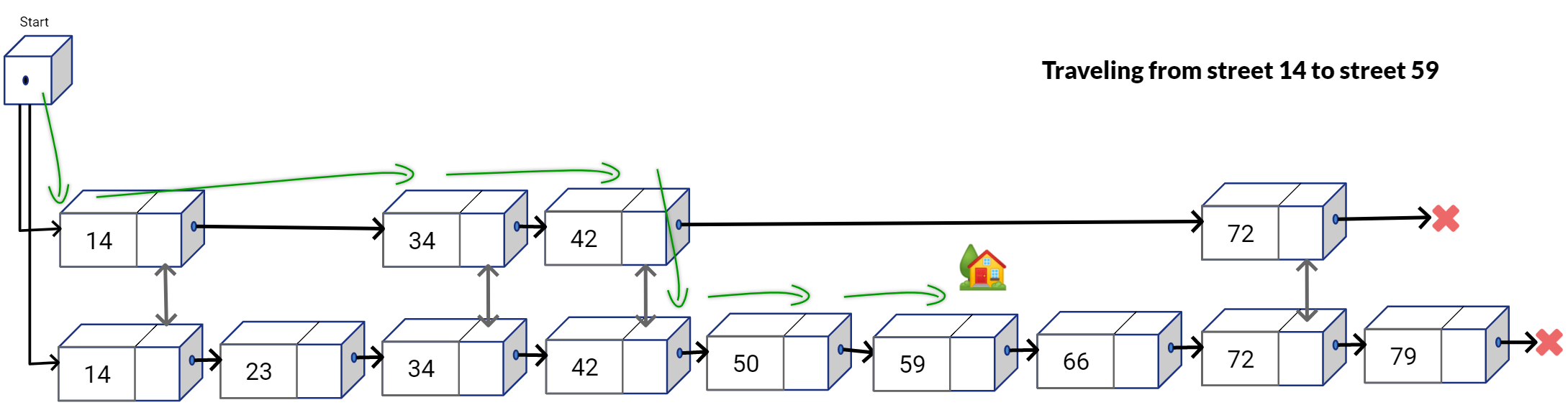
As you would notice, by taking the express route you would be able to skip some stations along the way and maybe even reach the destination much faster compared to taking the local train from a original stop and traveling each station one by one to reach a destination stop. This is exactly the core idea behind Skip List. With Skip Lists, we introduce redundant travel paths at the cost of additional space, but the additional travel paths have lesser and lesser number of “stops” such that the linear traversal is much faster if we travel in those additional lanes.

Skip Lists - Basics

Let’s now build the concept of Skips Lists from bottom to top.

Assume that we have a Doubly Linked List which is unsorted. What do you think would be the search complexity for this list?

Search would be done in O(n), because you would have to traverse the list linearly to find your target node.

Let’s assume that the list is now sorted as shown below. What do you think is the search complexity now?

Well, it’s still O(n). Even if it sorted, the linked list structure doesn’t provide us random access, hence we can’t simply calculate the next middle index and access that middle node in O(1).

Now, let’s put our “express line” on top of the existing structure. We are going to create a second Doubly Linked List and place the second list above of the first list such that each node has four reference to neighboring nodes: left, right, above, below.

which can be visualized as:

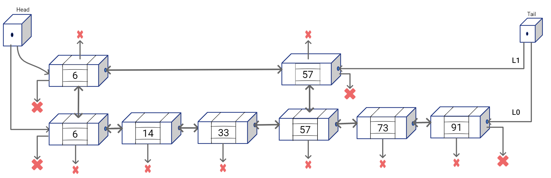
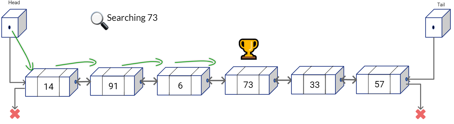
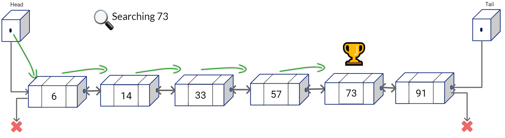
Now given this Skip Lists structure, you can find the number 73 with lesser number of comparison operations. You can start traversing from the top list first, and at every node see if the next node overshoots the value that you are looking for. If it doesn’t simply go the next node in the list on the top, else go to the list on the bottom and continue your linear search in the bottom list.

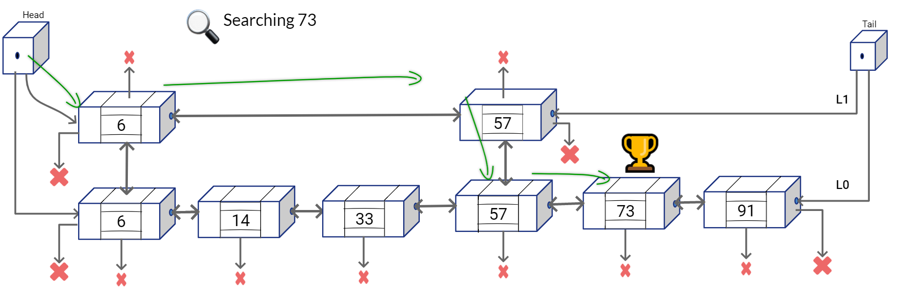
We can summarize the searching approach in a simple algorithm.

So what is the kind of search cost we are looking at?

We would want to travel the length of L1 as much as possible because that gives us skips over unnecessary comparisons. And eventually we may go down to L0 and traverse a portion of it. The idea is to uniformly disperse the nodes in the top lane.

It can be mathematically shown¹ that if the cardinality of the bottom list is n (i.e. it has n nodes), we will get an optimal solution if we have \(\sqrt{n}\) nodes in the top layer.

So, if the nodes are optimally dispersed, theoretically the structure gives us our favorite logarithmic complexity 🙂 (Although in implementation when we use randomization to insert the nodes, things get a little tricky).

Now think of the structure we have created. At the bottom we have n nodes, the layer on top has interspersed \(\frac{n}{2}\) nodes and the layer above it has \(\frac{n}{4}\) nodes. Do you how this structure looks quite similar to a tree? We just need to figure out how “balancing” works in this tree (hint: it’s probabilistic).

Skip List - Definition

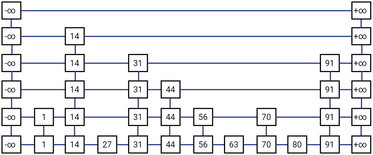
Skip List S consists of a series of lists {\(S_0,S_1 .. S_h\)} such that each list \(S_i\) stores a subset of the items sorted by increasing keys.

Let’s first simplify the visualization for our nodes and connection in Skip List.

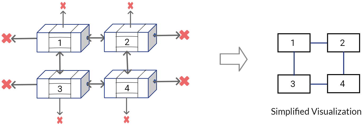
A standard, simplified Skip List would look like this:

Now, let’s see how some of the basic operations are performed on a Skip List.

Searching in Skip List

Searching in a Skip List in straightforward. We have already seen an example above with two lists. We can extend the same approach to a Skip List with h lists. We will simply start with the leftmost node in the list on top. Go down if the next value in the same list is greater than the one we are looking for, go right otherwise.

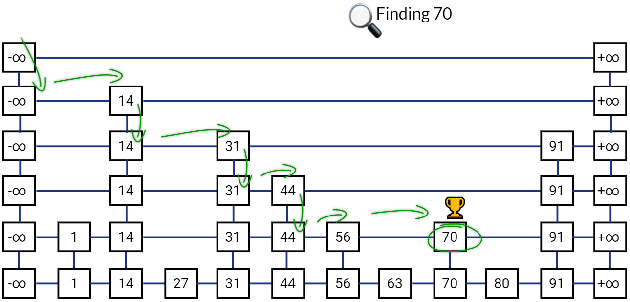
The main idea is again to skip comparisons with as many keys as possible, while compromising a little on the extra storage required in the additional lists containing subset of all keys. On average, “expected” Search complexity for Skip List is O(log(n))

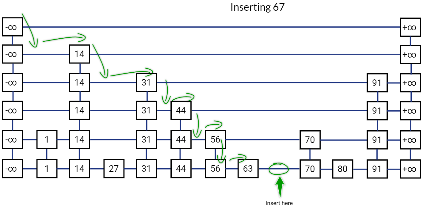
Inserting in Skip List

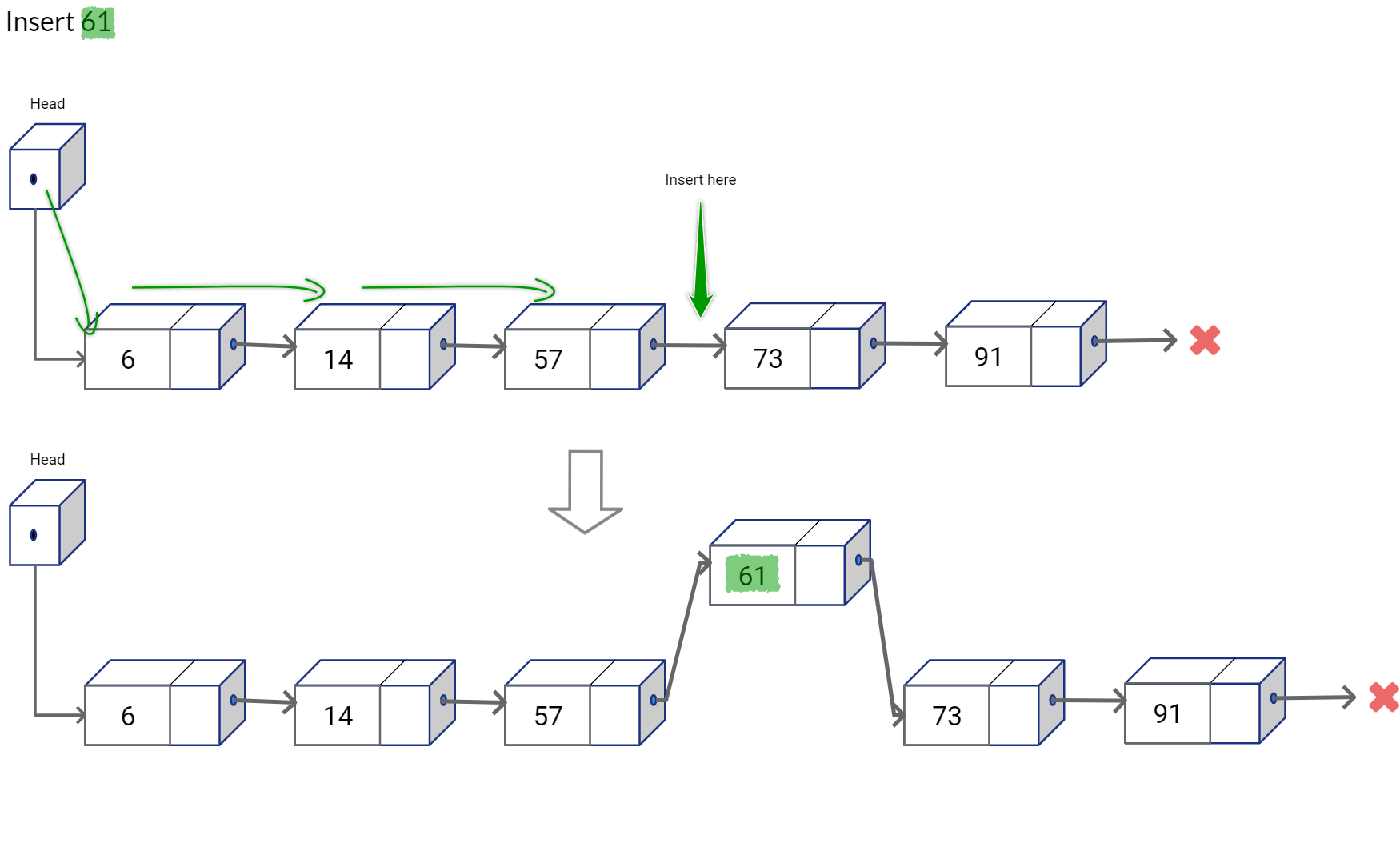
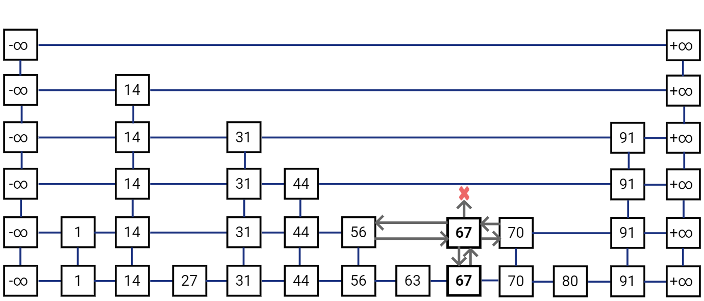
To insert a new node, we would first find the location where this new key should be inserted in the list at the very bottom. This can be simply done be re-using the search logic, we start traversing to the right from the list on top and we go one step down if the next item is bigger than the key that we want to insert, else go right. Once we reach at a position in bottom list where we can’t go more to the right, we insert the new value on the right side of that position.

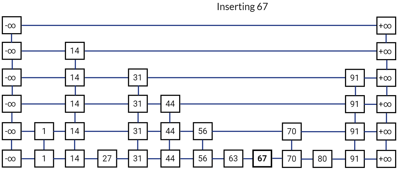
Skip List after inserting 67:

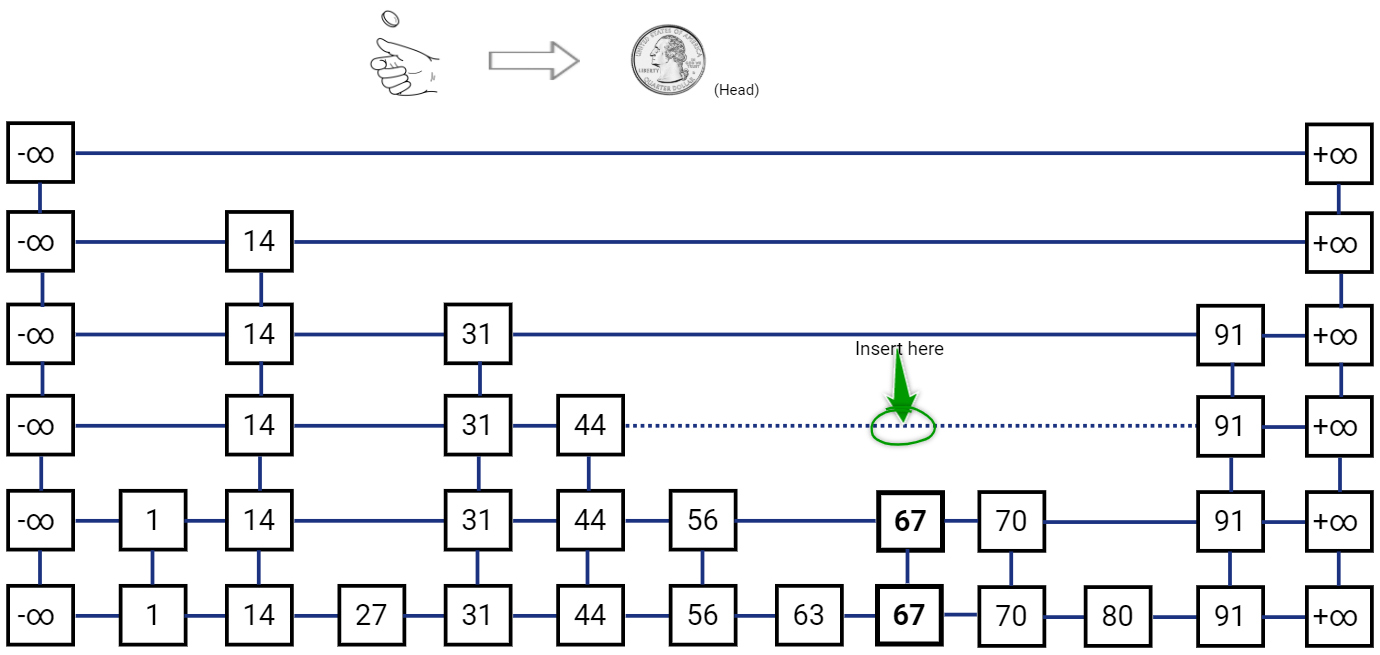
Now comes the probabilistic part, after inserting the new node in the list \(L_i\) we have to also insert the node in list above it, i.e. list \(L_{i+1}\) with probability \(\frac{1}{2}\). We do this with a simple coin toss, such that if we get a head we insert the node in the list \(L_{i+1}\) and toss the coin again, we stop when we get a tail. We may repeat the coin toss till we keep getting heads, even if we have to insert a new layer (list) at the top.

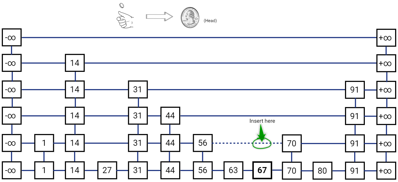
Note that we also need to “re-hook” the links for the newly inserted node. The new node needs to have it’s ‘below’ reference pointing to the node below, and the node below would have ‘above’ reference pointer to the new node. To find the ’left’ neighbor for the new node, we simply traverse towards left from the node below it and return ‘above’ pointer from a node for which ‘above’ pointer is not null. The ‘right’ reference of the ’left’ neighbor is used to update the ‘right’ reference of the new node. Also, the ’left’ reference for the new node’s right neighbor is also updated to the new node. This re-hooking operation is actually pretty easy to implement with Linked Lists.

Let’s toss the coin again.

Last toss gave us another Head, so let’s toss the coin again.

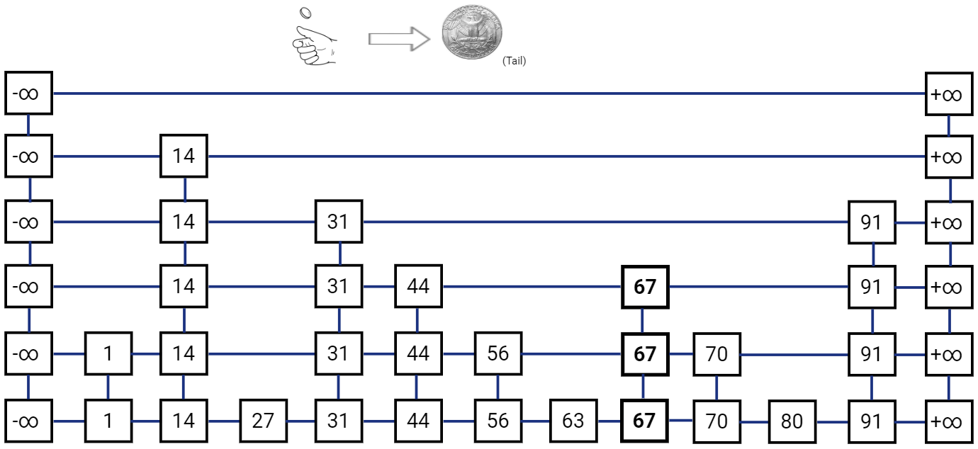
We got a Tail this time, so no more insertions are required.

As you see the probability of a node also getting inserted in the layer above it get reduced by half after every layer. Still, there is a worst case possibility that you would keep getting Heads indefinitely, although the probability of that happening is extremely small. To avoid such cases when you may get a large number of heads sequentially, you could also use a termination condition where you stop inserting if you reach a predefined threshold for the number of layers (height) or a predefined threshold for the number of nodes in a specific layer. Although the expected time complexity would still be O(log(n)) for all operations.

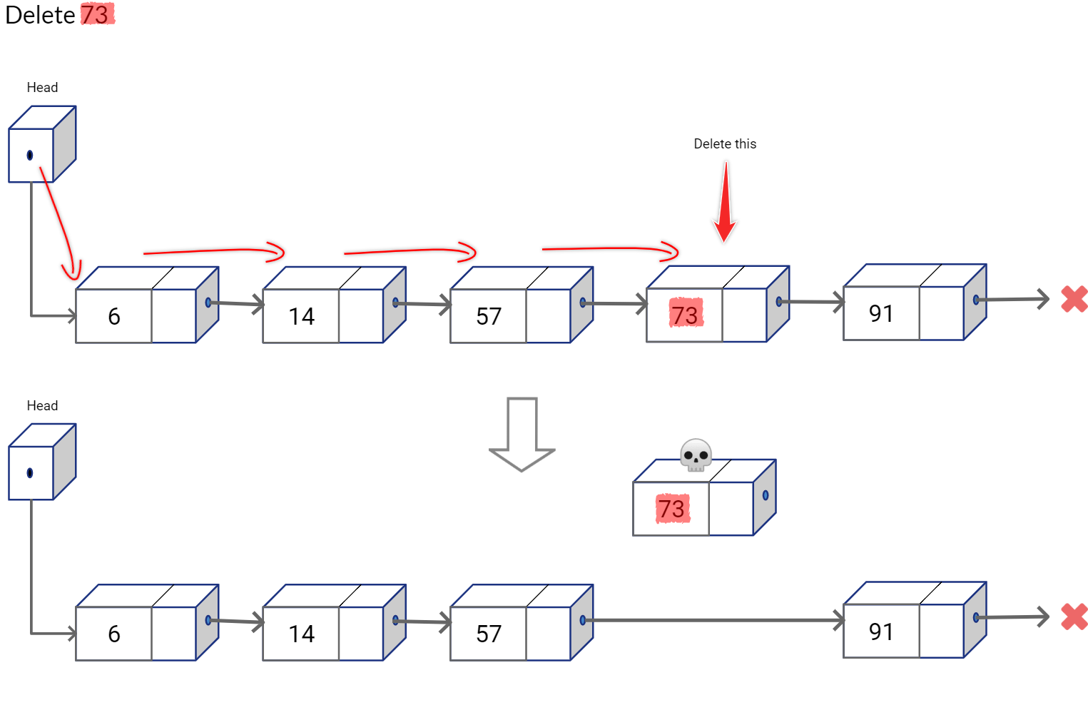
Deletion in Skip List

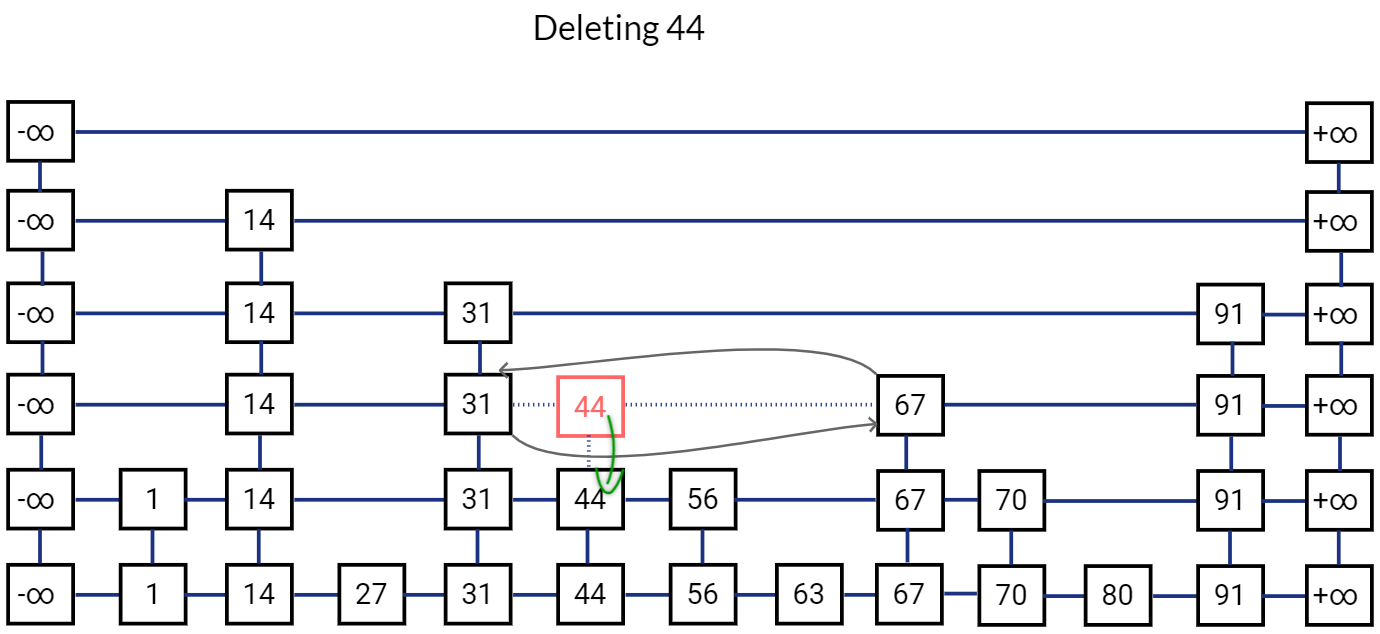
Deletion operation in Skip List is pretty straightforward. We first perform search operation to find the location of the node. If we find the node, we simply delete it at all levels. Before deleting a node, we simply ensure that no other node is pointing to it.

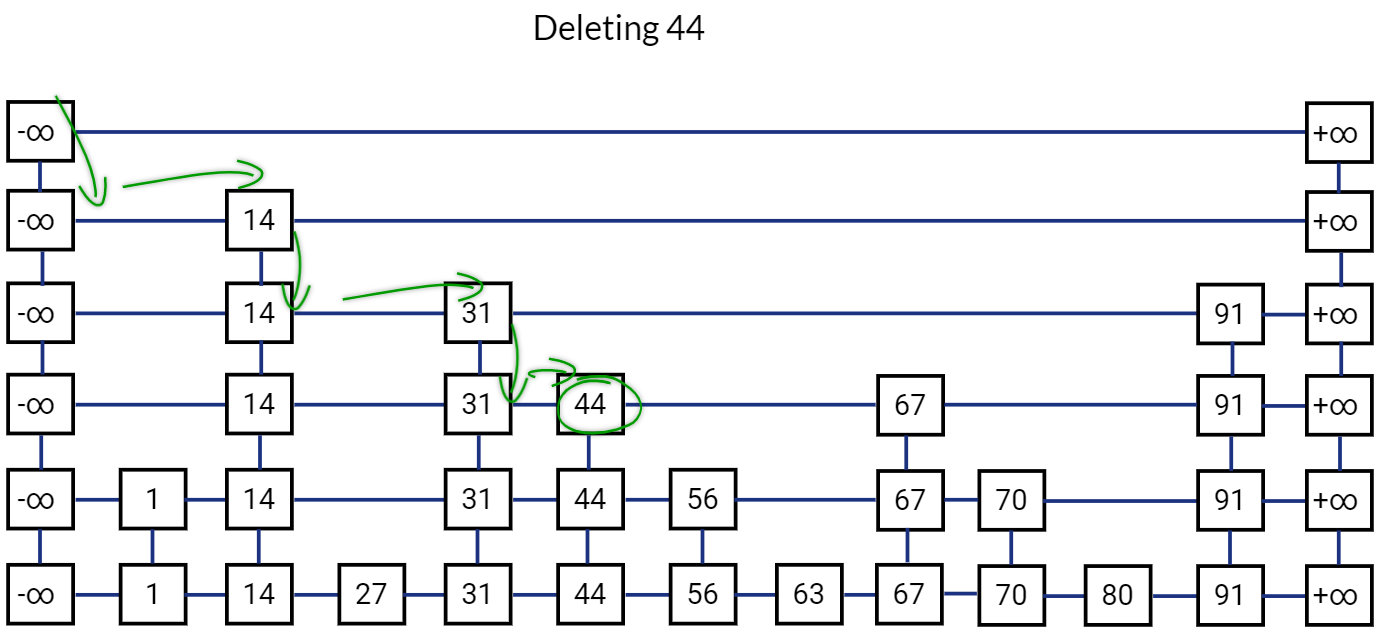
Release all references to this node. And move to the node below it.

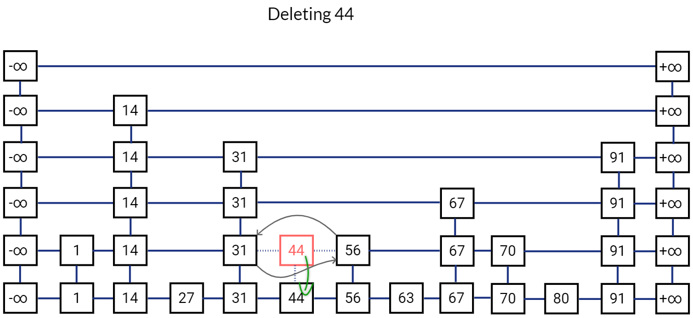
Remove all references to this node and release it. Move to the node below in the bottom list.

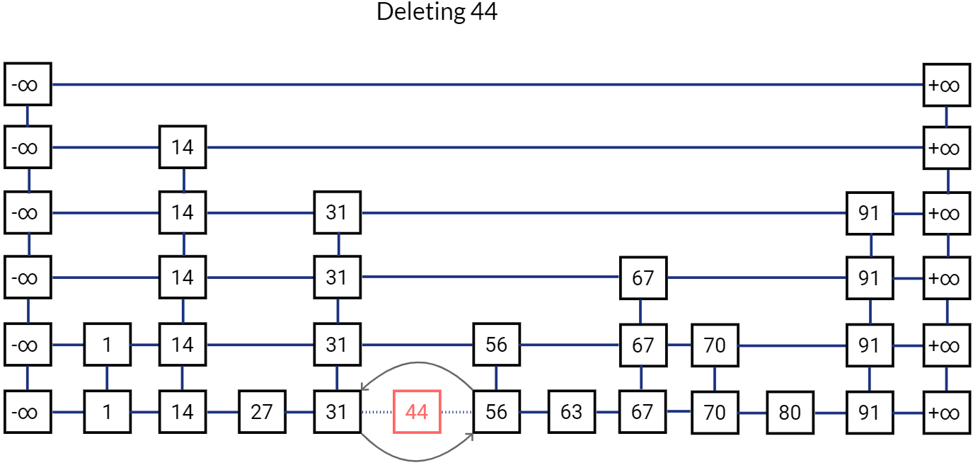
Release this node as well.

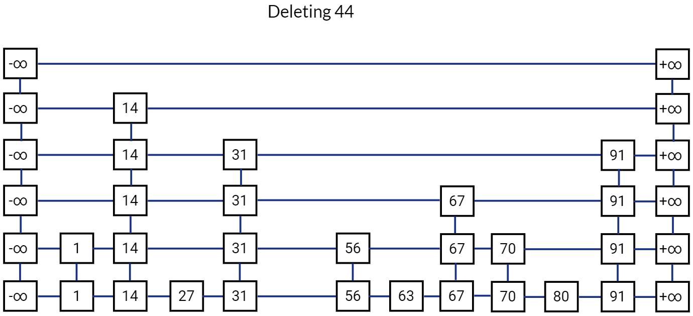
This is how our Skip List looks like after deletion.

Conclusion

In this article we saw how Skip List is a probabilistic data structure that loosely resembles a balanced binary tree. It is also easy to implement and very fast as the search, insert, delete operations have an expected time complexity of O(log(n)), along with O(n) expected space complexity. in next article, I will introduce a practical application of Skip List and explain how Twitter used Skip List to get a huge improvement in their search indexing latency.

Reference and Further Reading